Model based Subsampling for Bike Sharing Data

# Load the R packages
library(NeEDS4BigData)

## Error in get(paste0(generic, ".", class), envir = get_method_env()) : 
##   object 'type_sum.accel' not found

library(ggplot2)
library(ggpubr)
library(kableExtra)
library(tidyr)
library(psych)
library(gam)

# Theme for plots
Theme_special<-function(){
  theme(legend.key.width= unit(1,"cm"),
        axis.text.x= element_text(color= "black", size= 12, angle= 30, hjust=0.75),
        axis.text.y= element_text(color= "black", size= 12), 
        strip.text= element_text(colour= "black", size= 12, face= "bold"),
        panel.grid.minor.x= element_blank(),
        axis.title= element_text(color= "black", face= "bold", size= 12),
        legend.text= element_text(color= "black", size= 11),
        legend.position= "bottom",
        legend.margin= margin(0,0,0,0),
        legend.box.margin= margin(-1,-2,-1,-2)) 
}

Fanaee-T and Gama (2013) collected data to understand the bike sharing demands under the rental and return process. The data contains \(4\) columns and has \(17,379\) observations, first column is the response variable and the rest are covariates. We consider the covariates a) temperature (\(x_1\)), b) humidity (\(x_2\)) and c) wind speed (\(x_3\)) to model the response, the number of bikes rented hourly. The covariates are scaled to be mean of zero and variance of one. For the given data subsampling methods are implemented assuming the main effects model can describe the data.

# Selecting 100% of the big data and prepare it
Original_Data<-cbind(Bike_sharing[,1],1,Bike_sharing[,-1])
colnames(Original_Data)<-c("Y",paste0("X",0:ncol(Original_Data[,-c(1,2)])))

# Scaling the covariate data
for (j in 3:5) {
  Original_Data[,j]<-scale(Original_Data[,j])
}
head(Bike_sharing) %>% 
  kable(format = "html",
        caption = "First few observations of the bike sharing data.")

First few observations of the bike sharing data.
Rented_Bikes	Temperature	Humidity	Windspeed
16	0.24	0.81	0.0000
40	0.22	0.80	0.0000
32	0.22	0.80	0.0000
13	0.24	0.75	0.0000
1	0.24	0.75	0.0000
1	0.24	0.75	0.0896

# Setting the sample sizes
N<-nrow(Original_Data); M<-250; k<-seq(8,20,by=2)*100; rep_k<-rep(k,each=M)

Based on this model the methods random sampling, leverage sampling (Ma, Mahoney, and Yu 2014; Ma and Sun 2015), \(A\)- and \(L\)-optimality subsampling (Ai et al. 2021; Yao and Wang 2021) and \(A\)-optimality subsampling with response constraint (Zhang, Ning, and Ruppert 2021) are implemented on the big data.

# define colors, shapes, line types for the methods
Method_Names<-c("A-Optimality","L-Optimality","A-Optimality MC",
                "Shrinkage Leverage","Basic Leverage","Unweighted Leverage",
                "Random Sampling")
Method_Colour<-c("#BBFFBB","#50FF50","#00BB00",
                 "#F76D5E","#D82632","#A50021","#000000")
Method_Shape_Types<-c(rep(17,3),rep(4,3),16)

The obtained samples and their respective model parameter estimates are over \(M=250\) simulations across different sample sizes \(k=(800,\ldots,2000)\). We set the initial sample size of \(r1=400\) for the methods that requires a random sample. From the final samples, model parameters of the assume model are estimated. These estimated model parameters are compared with the estimated model parameters of the full big data through the mean squared error \(MSE(\tilde{\beta}_k,\hat{\beta})=\frac{1}{MJ}\sum_{i=1}^M \sum_{j=1}^J(\tilde{\beta}_{k,j} - \hat{\beta}_j)^2\). Here, \(\tilde{\beta}_k\) is the estimated model parameters from the sample of size \(k\) and \(\hat{\beta}\) is the estimated model parameters from the full big data, while \(j\) is index of the model parameter.

Random sampling

Below is the code for this implementation.

# Random sampling
Final_Beta_RS<-matrix(nrow = length(k)*M,ncol = ncol(Original_Data[,-1])+1)
for (i in 1:length(rep_k)) {
  Temp_Data<-Original_Data[sample(1:N,rep_k[i]),]
  glm(Y~.-1,data=Temp_Data,family="poisson")->Results
  Final_Beta_RS[i,]<-c(rep_k[i],coefficients(Results))
  if(i==length(rep_k)){print("All simulations completed for random sampling")}
}

## [1] "All simulations completed for random sampling"

Final_Beta_RS<-cbind.data.frame("Random Sampling",Final_Beta_RS)
colnames(Final_Beta_RS)<-c("Method","Sample",paste0("Beta",0:3))

Leverage sampling

# Leverage sampling 
## we set the shrinkage value of S_alpha=0.9
NeEDS4BigData::LeverageSampling(r=rep_k,Y=as.matrix(Original_Data[,1]),
                                X=as.matrix(Original_Data[,-1]),N=N,
                                S_alpha = 0.9,family = "poisson")->Results

## Basic and shrinkage leverage probabilities calculated.

## Sampling completed.

Final_Beta_LS<-Results$Beta_Estimates
colnames(Final_Beta_LS)<-c("Method","Sample",paste0("Beta",0:3))

A- and L-optimality subsampling

# A- and L-optimality subsampling for GLM
NeEDS4BigData::ALoptimalGLMSub(r1=400,r2=rep_k,
                               Y=as.matrix(Original_Data[,1]),
                               X=as.matrix(Original_Data[,-1]),
                               N=N,family = "poisson")->Results

## Step 1 of the algorithm completed.

## Step 2 of the algorithm completed.

Final_Beta_ALoptGLM<-Results$Beta_Estimates
colnames(Final_Beta_ALoptGLM)<-c("Method","Sample",paste0("Beta",0:3))

A-optimality subsampling with measurement constraints

# A-optimality subsampling without response
NeEDS4BigData::AoptimalMCGLMSub(r1=400,r2=rep_k,
                                Y=as.matrix(Original_Data[,1]),
                                X=as.matrix(Original_Data[,-1]),
                                N=N,family="poisson")->Results

## Step 1 of the algorithm completed.

## Step 2 of the algorithm completed.

Final_Beta_AoptMCGLM<-Results$Beta_Estimates
Final_Beta_AoptMCGLM$Method<-rep("A-Optimality MC",nrow(Final_Beta_AoptMCGLM))
colnames(Final_Beta_AoptMCGLM)<-c("Method","Sample",paste0("Beta",0:3))

Summary

# Summarising Results of Scenario one
Final_Beta<-rbind(Final_Beta_RS,Final_Beta_LS,
                  Final_Beta_ALoptGLM,Final_Beta_AoptMCGLM)

# Obtaining the model parameter estimates for the full big data model
glm(Y~.-1,data = Original_Data,family="poisson")->All_Results
coefficients(All_Results)->All_Beta
matrix(rep(All_Beta,by=nrow(Final_Beta)),nrow = nrow(Final_Beta),
       ncol = ncol(Final_Beta[,-c(1,2)]),byrow = TRUE)->All_Beta

remove(Final_Beta_RS,Final_Beta_LS,Final_Beta_ALoptGLM,
       Final_Beta_AoptMCGLM,Temp_Data,Results,All_Results)

The mean squared error is plotted below.

# Obtain the mean squared error for the model parameter estimates
MSE_Beta<-data.frame("Method"=Final_Beta$Method,
                     "Sample"=Final_Beta$Sample,
                     "SE"=rowSums((All_Beta - Final_Beta[,-c(1,2)])^2)) 

MSE_Beta$Method<-factor(MSE_Beta$Method,levels = Method_Names,labels = Method_Names)

Mean_Data <- MSE_Beta |>
    group_by(Method,Sample) |>
    dplyr::summarise(Mean = mean(SE),
                     min=quantile(SE,0.05),
                     max=quantile(SE,0.95), .groups = "drop")

# Plot for the mean squared error with all methods
ggplot(data=Mean_Data,aes(x=factor(Sample),y=Mean,color=Method,shape=Method))+
  xlab("Sample Size")+ylab("Squared Error")+
  geom_point(size=3,position = position_dodge(width = 0.5))+
  geom_line(data=Mean_Data,aes(x=factor(Sample),y=Mean,group=Method,color=Method),
            position = position_dodge(width = 0.5))+
  geom_errorbar(data=Mean_Data,aes(ymin=min,ymax=max),
                width=0.3,position = position_dodge(width = 0.5))+
  scale_color_manual(values = Method_Colour)+
  scale_shape_manual(values = Method_Shape_Types)+
  theme_bw()+Theme_special()+
  guides(colour = guide_legend(nrow = 3))->p1

# Plot for the mean squared error with all methods except unweighted leverage
ggplot(data=Mean_Data[Mean_Data$Method != "Unweighted Leverage",],
       aes(x=factor(Sample),y=Mean,color=Method,shape=Method))+
  xlab("Sample Size")+ylab("Squared Error")+
  geom_point(size=3,position = position_dodge(width = 0.5))+
  geom_line(data=Mean_Data[Mean_Data$Method != "Unweighted Leverage",],
            aes(x=factor(Sample),y=Mean,group=Method,color=Method),
            position = position_dodge(width = 0.5))+
  geom_errorbar(data=Mean_Data[Mean_Data$Method != "Unweighted Leverage",],
                aes(ymin=min,ymax=max),width=0.3,
                position = position_dodge(width = 0.5))+
  scale_color_manual(values = Method_Colour[-7])+
  scale_shape_manual(values = Method_Shape_Types[-7])+
  theme_bw()+Theme_special()+
  guides(colour = guide_legend(nrow = 3))->p2

ggarrange(p1,p2,nrow = 2,ncol = 1,labels = "auto")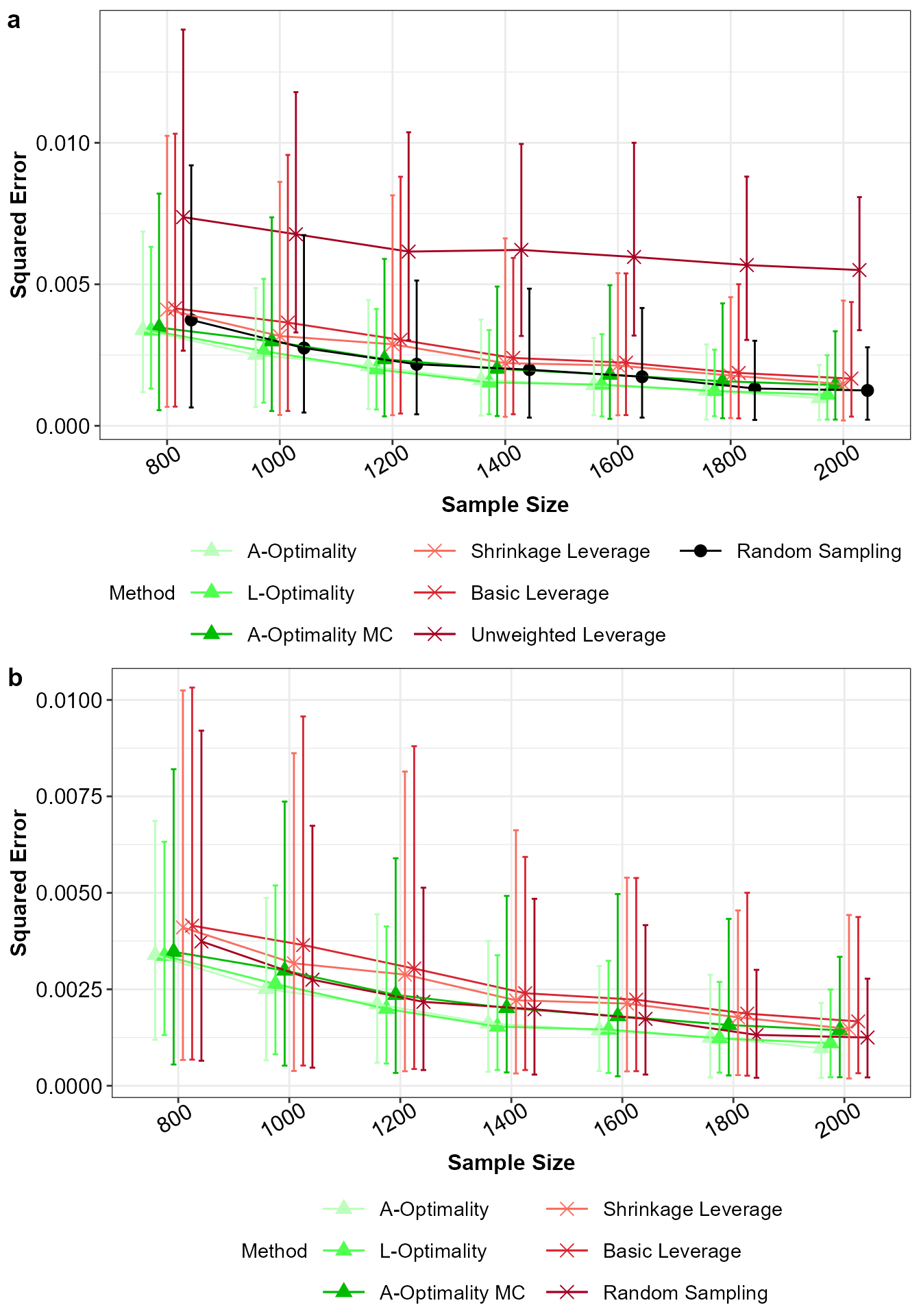

Mean squared error for a) all the subsampling methods and b) without unweighted leverage sampling, with 5% and 95% percentile intervals.

References

Ai, Mingyao, Jun Yu, Huiming Zhang, and HaiYing Wang. 2021. “Optimal Subsampling Algorithms for Big Data Regressions.” Statistica Sinica 31 (2): 749–72.

Fanaee-T, Hadi, and J Gama. 2013. “Bike Sharing Data Set.” UCI Machine Learning Repository.

Ma, Ping, Michael Mahoney, and Bin Yu. 2014. “A Statistical Perspective on Algorithmic Leveraging.” In International Conference on Machine Learning, 91–99. PMLR.

Ma, Ping, and Xiaoxiao Sun. 2015. “Leveraging for Big Data Regression.” Wiley Interdisciplinary Reviews: Computational Statistics 7 (1): 70–76.

Yao, Yaqiong, and HaiYing Wang. 2021. “A Review on Optimal Subsampling Methods for Massive Datasets.” Journal of Data Science 19 (1): 151–72.