Model robust and potential model misspecification for Bike Sharing Data
Source:vignettes/MR_MM_Poisson_Reg_Bike_Sharing.Rmd
MR_MM_Poisson_Reg_Bike_Sharing.Rmd
# Load the R packages
library(NeEDS4BigData)
## Error in get(paste0(generic, ".", class), envir = get_method_env()) :
## object 'type_sum.accel' not found
library(ggplot2)
library(ggpubr)
library(kableExtra)
library(tidyr)
library(psych)
library(gam)

# Theme for plots
Theme_special<-function(){
  theme(legend.key.width= unit(1,"cm"),
        axis.text.x= element_text(color= "black", size= 12, angle= 30, hjust=0.75),
        axis.text.y= element_text(color= "black", size= 12),
        strip.text= element_text(colour= "black", size= 12, face= "bold"),
        panel.grid.minor.x= element_blank(),
        axis.title= element_text(color= "black", face= "bold", size= 12),
        legend.text= element_text(color= "black", size= 11),
        legend.position= "bottom",
        legend.margin= margin(0,0,0,0),
        legend.box.margin= margin(-1,-2,-1,-2))
}
Understanding the bike sharing data
Fanaee-T and Gama (2013) collected data to understand the bike sharing demands under the rental and return process. The data contains \(4\) columns and has \(17,379\) observations, first column is the response variable and the rest are covariates. We consider the covariates a) temperature (\(x_1\)), b) humidity (\(x_2\)) and c) windspeed (\(x_3\)) to model the response, the number of bikes rented hourly. The covariates are scaled to be mean of zero and variance of one.
Given data is analysed under two different scenarios,
- model robust or average subsampling methods assuming that a set of models can describe the data.
- subsampling method assuming the main effects model is potentially misspecified.
# Selecting 100% of the big data and prepare it
Original_Data<-cbind(Bike_sharing[,1],1,Bike_sharing[,-1])
colnames(Original_Data)<-c("Y",paste0("X",0:ncol(Original_Data[,-c(1,2)])))

# Scaling the covariate data
for (j in 3:5) {
  Original_Data[,j]<-scale(Original_Data[,j])
}
head(Bike_sharing) %>%
  kable(format = "html",
caption = "First few observations of the bike sharing data.")| Rented_Bikes | Temperature | Humidity | Windspeed |
|---|---|---|---|
| 16 | 0.24 | 0.81 | 0.0000 |
| 40 | 0.22 | 0.80 | 0.0000 |
| 32 | 0.22 | 0.80 | 0.0000 |
| 13 | 0.24 | 0.75 | 0.0000 |
| 1 | 0.24 | 0.75 | 0.0000 |
| 1 | 0.24 | 0.75 | 0.0896 |
# Setting the sample sizes
N<-nrow(Original_Data); M<-250; k<-seq(8,20,by=2)*100; rep_k<-rep(k,each=M)
Model robust or average subsampling
The method \(A\)- and \(L\)-optimality of model robust or average
subsampling (Mahendran, Thompson, and McGree
2023) is compared against the \(A\)- and \(L\)-optimality subsampling (Ai et al. 2021; Yao and Wang 2021) method. Here
five models are selected out of eight models, which are 1) main effects
model (\(\beta_0+\beta_1X_1+\beta_2X_2+\beta_3X_3\)),
2-4) main effects model with the squared term of each covariate (\(X^2_1 / X^2_2 / X^2_3\)), 5-7) main effects
model with two squared terms (\(X^2_1+X^2_2 /
X^2_1+X^2_3 / X^2_2+X^2_3\)) and 8) main effects model with all
squared terms. The five models are selected based on the smallest AIC
values.
For each model \(j\) the mean squared
error of the model parameters \(MSE_l(\tilde{\beta}_k,\hat{\beta})=\frac{1}{MJ}
\sum_{i=1}^M \sum_{j=1}^J (\tilde{\beta}_{k,j} -
\hat{\beta}_j)^2\) are calculated for the \(M=250\) simulations across the sample sizes
\(k=(800,\ldots,2000)\) and the initial
sample size is \(r1=400\). Here, for
the \(l\)-th model \(\tilde{\beta}_k\) is the estimated model
parameters from the sample of size \(k\) and \(\hat{\beta}\) is the estimated model
parameters from the full big data, while \(j\) is index of the model parameter.
# Define the subsampling methods and their respective colours, shapes and line types
Method_Names<-c("A-Optimality","L-Optimality","A-Optimality MR","L-Optimality MR")
Method_Colour<-c("#D82632","#A50021","#50FF50","#00BB00")
Method_Shape_Types<-c(rep(8,2),rep(17,2))

# Preparing the data for the model average method with squared terms
No_of_Variables<-ncol(Original_Data[,-c(1,2)])
Squared_Terms<-paste0("X",1:No_of_Variables,"^2")
term_no <- 2
All_Models <- list(c("X0",paste0("X",1:No_of_Variables)))

Original_Data_ModelRobust<-cbind(Original_Data,Original_Data[,-c(1,2)]^2)
colnames(Original_Data_ModelRobust)<-c("Y","X0",paste0("X",1:No_of_Variables),
                                       paste0("X",1:No_of_Variables,"^2"))
Temp_Data<-Original_Data_ModelRobust[sample(1:N,1000),]

AIC_Values<-NULL
model <- glm(Y~.-1, family = "poisson",
             data = Temp_Data[,c("Y","X0",paste0("X",1:No_of_Variables))])
AIC_Values[1]<-AIC(model)
for (i in 1:No_of_Variables)
{
  x <- as.vector(combn(Squared_Terms,i,simplify = FALSE))
  for(j in 1:length(x))
  {
    All_Models[[term_no]] <- c("X0",paste0("X",1:No_of_Variables),x[[j]])
    temp_data<-as.data.frame(Temp_Data[,c("Y",All_Models[[term_no]])])
    model <- glm(Y~.-1, data = temp_data,family = "poisson")
    AIC_Values[term_no]<-AIC(model)
    term_no <- term_no+1
  }
}

Model_Set<-5
Best_Indices <- order(AIC_Values,decreasing = FALSE)[1:Model_Set]
Model_Apriori<-rep(1/Model_Set,Model_Set)
All_Models<-All_Models[Best_Indices]
names(All_Models)<-paste0("Model_",1:length(All_Models))
Covariates in the selected five models
- X0, X1, X2, X3, X1^2, X2^2, X3^2
- X0, X1, X2, X3, X1^2, X2^2
- X0, X1, X2, X3, X1^2, X3^2
- X0, X1, X2, X3, X1^2
- X0, X1, X2, X3, X2^2, X3^2
A priori probabilities are equal
Consider for \(Q=5\) each model has an equal a priori probability (i.e \(\alpha_q=1/5,q=1,\ldots,5\)). Below is the code of implementation for this scenario.
All_Covariates<-colnames(Original_Data_ModelRobust)[-1]
# A- and L-optimality model robust subsampling for poisson regression
NeEDS4BigData::modelRobustPoiSub(r1=400,r2=rep_k,
                                 Y=as.matrix(Original_Data_ModelRobust[,1]),
                                 X=as.matrix(Original_Data_ModelRobust[,-1]),
                                 N=N,Apriori_probs=rep(1/Model_Set,Model_Set),
                                 All_Combinations = All_Models,
                                 All_Covariates = All_Covariates)->Results
## Step 1 of the algorithm completed.## Step 2 of the algorithm completed.
Final_Beta_modelRobust<-Results$Beta_Estimates

# Mean squared error and their respective plots for all five models
plot_list_MR<-list()
for (i in 1:length(All_Models)) {
  glm(Y~.-1,data=Original_Data_ModelRobust[,c("Y",All_Models[[i]])],
      family="poisson")->All_Results
  All_Beta<-coefficients(All_Results)

  matrix(rep(All_Beta,by=nrow(Final_Beta_modelRobust[[i]])),
         nrow = nrow(Final_Beta_modelRobust[[i]]),
         ncol = ncol(Final_Beta_modelRobust[[i]][,-c(1,2)]),byrow = TRUE)->All_Beta

  MSE_Beta_MR<-data.frame("Method"=Final_Beta_modelRobust[[i]]$Method,
                          "Sample"=Final_Beta_modelRobust[[i]]$r2,
                          "SE"=rowSums((All_Beta -
                                        Final_Beta_modelRobust[[i]][,-c(1,2)])^2))

  Mean_Data_MR <- MSE_Beta_MR |>
    group_by(Method,Sample) |>
    dplyr::summarise(Mean = mean(SE),
                     min=quantile(SE,0.05),
                     max=quantile(SE,0.95), .groups = "drop")

  ggplot(Mean_Data_MR,aes(x=factor(Sample),y=Mean,color=Method,shape=Method))+
    xlab("Sample size")+ylab("Squared Error")+
    geom_point(size=3,position = position_dodge(width = 0.5))+
    geom_line(data=Mean_Data_MR,aes(x=factor(Sample),y=Mean,group=Method,color=Method),
            position = position_dodge(width = 0.5))+
    geom_errorbar(data=Mean_Data_MR,aes(ymin=min,ymax=max),
                width=0.3,position = position_dodge(width = 0.5))+
    ggtitle(paste0("Model ",i))+
    scale_color_manual(values = Method_Colour)+
    scale_shape_manual(values= Method_Shape_Types)+
    theme_bw()+guides(colour= guide_legend(nrow = 2))+
    Theme_special()->plot_list_MR[[i]]
}

ggarrange(plotlist = plot_list_MR,nrow = 3,ncol = 2,labels = "auto",
          legend = "bottom",common.legend = TRUE)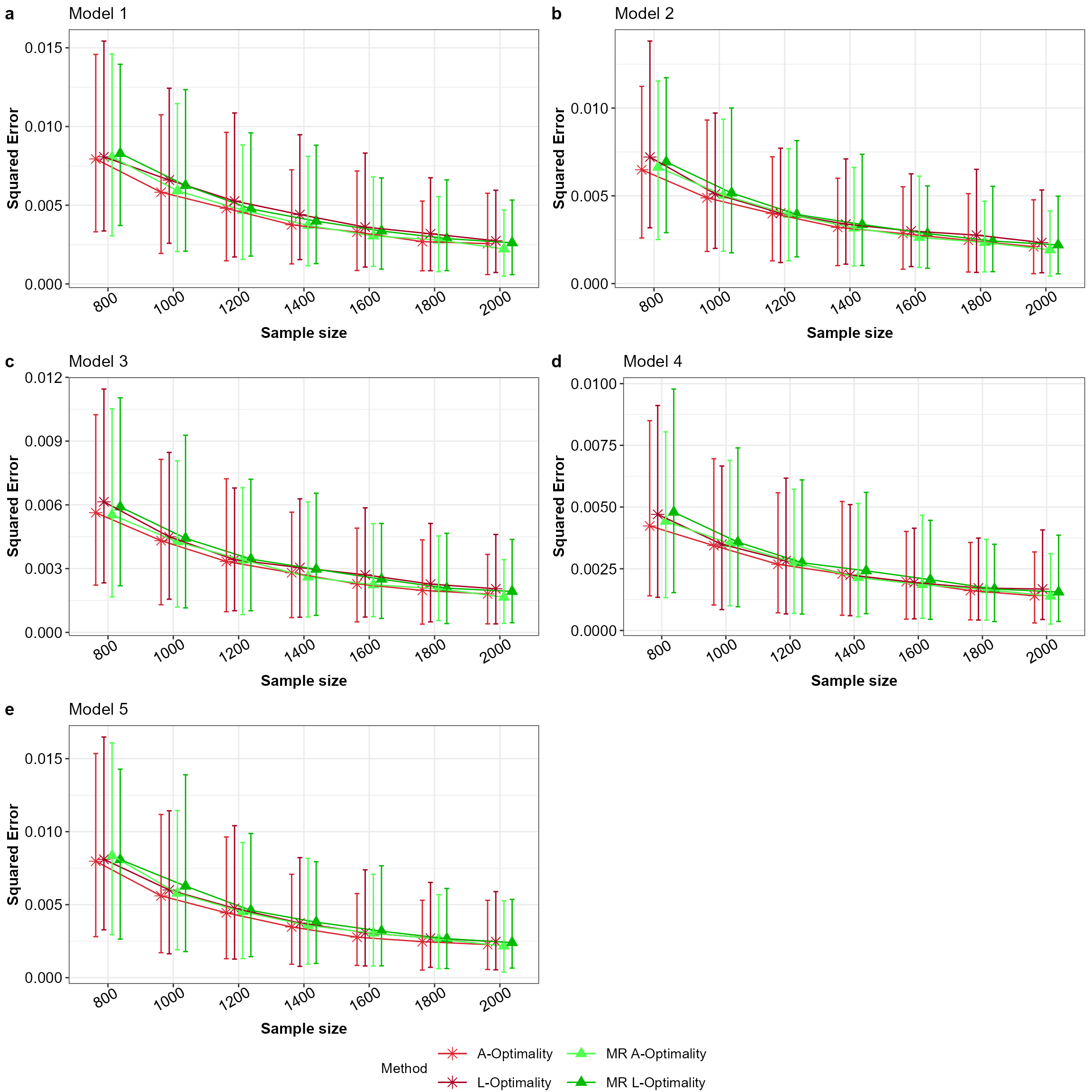
Mean squared error for all the models with equal apriori in the order a to e for Model 1 to 5 across the subsampling methods under comparison.
Main effects model is potentially misspecified
The final and third scenario is for comparison of the subsampling method under the assumption that the main effects model is potentially misspecified against the \(A\)- and \(L\)-optimality subsampling method. Under the subsampling method that accounts for potential model misspecification we take the scaling factor of \(\alpha=10\). As in scenario one an two the number of simulations and the sample sizes stay the same. We compare the mean squared error of the estimated model parameters, however as we assume the model is potentially misspecified the asymptotic approximation of the mean squared error from the predictions are calculated as well. Below is the code for this implementation.
# Define the subsampling methods and their respective colors, shapes and line types
Method_Names<-c("A-Optimality","L-Optimality","L1-Optimality","RLmAMSE",
                "RLmAMSE Log Odds 10","RLmAMSE Power 10")
Method_Colour<-c("#D82632","#A50021","greenyellow","#BBFFBB","#50FF50","#00BB00")
Method_Shape_Types<-c(rep(8,3),rep(17,3))

# A- and L-optimality and RLmAMSE model misspecified subsampling for poisson regression
NeEDS4BigData::modelMissPoiSub(r1=400,r2=rep_k,
                               Y=as.matrix(Original_Data[,1]),
                               X=as.matrix(Original_Data[,-1]),
                               N=N,Alpha=10, proportion = 1)->Results
## 50% or >=50% of the big data is used to help find AMSE for the subsamples,
## this could take some time.## Step 1 of the algorithm completed.## Step 2 of the algorithm completed.
Final_Beta_modelMiss<-Results$Beta_Estimates
Final_AMSE_modelMiss<-Results$AMSE_Estimates

glm(Y~.-1,data=Original_Data,family="poisson")->All_Results
All_Beta<-coefficients(All_Results)

matrix(rep(All_Beta,by=nrow(Final_Beta_modelMiss)),nrow = nrow(Final_Beta_modelMiss),
       ncol = ncol(Final_Beta_modelMiss[,-c(1,2)]),byrow = TRUE)->All_Beta

# Plots for the mean squared error of the model parameter estimates
# and the AMSE for the main effects model
MSE_Beta_modelMiss<-data.frame("Method"=Final_Beta_modelMiss$Method,
                               "Sample"=Final_Beta_modelMiss$r2,
                               "SE"=rowSums((All_Beta -
                                              Final_Beta_modelMiss[,-c(1,2)])^2))

Mean_Data_MM <- MSE_Beta_modelMiss |>
  group_by(Method,Sample) |>
  dplyr::summarise(Mean = mean(SE),
                   min=quantile(SE,0.05),
                   max=quantile(SE,0.95), .groups = "drop")

ggplot(Mean_Data_MM,aes(x=factor(Sample),y=Mean,color=Method,shape=Method))+
  xlab("Sample size")+ylab("MSE")+
  geom_point(size=3,position = position_dodge(width = 0.5))+
  geom_line(data=Mean_Data_MM,aes(x=factor(Sample),y=Mean,group=Method,color=Method),
            position = position_dodge(width = 0.5))+
  geom_errorbar(data=Mean_Data_MM,aes(ymin=min,ymax=max),
                width=0.3,position = position_dodge(width = 0.5))+
  scale_color_manual(values = Method_Colour)+
  scale_shape_manual(values = Method_Shape_Types)+
  theme_bw()+guides(colour = guide_legend(nrow = 3))+Theme_special()->p1

Mean_AMSE<-Final_AMSE_modelMiss |> dplyr::group_by(r2,Method) |>
       dplyr::summarise(Mean=mean(AMSE),
                        min=quantile(AMSE,0.05),
                        max=quantile(AMSE,0.95),.groups ='drop')

ggplot(Mean_AMSE,aes(x=factor(r2),y=Mean,color=Method,shape=Method)) +
  geom_point(size=3,position = position_dodge(width = 0.5))+
  geom_line(data=Mean_AMSE,aes(x=factor(r2),y=Mean,group=Method,color=Method),
            position = position_dodge(width = 0.5))+
  geom_errorbar(data=Mean_AMSE,aes(ymin=min,ymax=max),
                width=0.3,position = position_dodge(width = 0.5))+
  xlab("Sample size")+ylab("Mean AMSE")+
  scale_color_manual(values = Method_Colour)+
  scale_shape_manual(values = Method_Shape_Types)+
  theme_bw()+guides(colour = guide_legend(nrow = 3))+Theme_special()->p2

ggarrange(p1,p2,nrow = 2,ncol = 1,labels = "auto")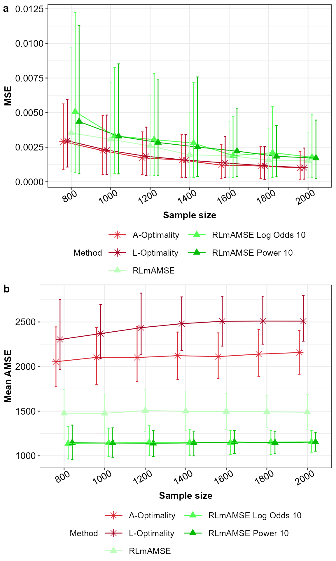
MSE for the model parameters (a) and AMSE (b) for the potentially misspecified main effects model across the subsampling methods under comparison, with 5% and 95% percentile intervals.