Benchmarking potential model-misspecification through subsampling functions
Source:vignettes/Benchmark_model_misspecification.Rmd
Benchmark_model_misspecification.Rmd## Error in get(paste0(generic, ".", class), envir = get_method_env()) :
## object 'type_sum.accel' not found
library(ggpubr)
library(tidyr)
library(dplyr)

# Theme for plots
Theme_special<-function(){
  theme(legend.key.width=unit(1,"cm"),
        axis.text.x = element_text(color = "black",size=14),
        axis.text.y = element_text(color = "black",size=14),
        strip.text = element_text(colour = "black",size = 16,face="bold"),
        panel.grid.minor.x = element_blank(),
        axis.title= element_text(color = "black",face = "bold",size = 14),
        legend.text = element_text(color = "black", size=16),
        legend.position = "bottom",
        legend.margin=margin(0,0,0,0),
        legend.box.margin=margin(-1,-2,-1,-2))
}

invisible(load("additionaldata/Results_Model_Misspecification.Rdata"))
Setup
The lm(), biglm(), glm(), and
bigglm() functions are benchmarked against the
model-misspecification subsampling functions. This benchmarking is
conducted across all three regression problems using a consistent setup
throughout. For large data sizes \(N =
\{10^4,5 \times 10^4,10^5,5 \times 10^5,10^6\}\), three different
covariate sizes \(\{5,10,25\}\), and
two different misspecification types \(\{1,2\}\), the functions were replicated
\(100\) times. When using the
model-misspecification subsampling functions, the initial subsample
sizes \(r_0=\{100,200,500\}\) were
selected based on the covariate sizes, while the final subsample size
was fixed at \(r_f=2500\). Further
based on the size of big data we set different proportion sizes to
estimate the AMSE, that is \(\{0.5,0.1,0.05,0.02,0.005\}\), such that
the sample size is \(5000\).
N_size<-c(1,5,10,50,100)*10000
N_size_labels<-c("10^4","5 x 10^4","10^5","5 x 10^5","10^6")
CS_size<-c(5,10,25)
MM_size<-c(1,2)
N_and_CS_size <- c(t(outer(CS_size, N_size_labels,
                           function(cs, n) paste0("N = ",n,
                                                  " and \nNumber of Covariates ",cs))))
This implementation was conducted on a high-performance computing system; however, the code for linear regression-related functions is shown below. Furthermore, it can be extended to logistic and Poisson regression using the relevant subsampling functions and model configurations.
# load the packages
library(NeEDS4BigData)
library(here)
library(biglm)
library(Rfast)

# indexes for N, covariate sizes and misspecification types
indexA <- as.numeric(Sys.getenv("indexA"))
indexB <- as.numeric(Sys.getenv("indexB"))
indexC <- as.numeric(Sys.getenv("indexC"))

# set N, covariate size and assign replicates
N_size<-c(1,5,10,50,100)*10000
Covariate_size<-c(5,10,25)
Replicates<-100

# set the initial and final subsample sizes,
# with the proportion values for AMSE calculation
r0<-c(1,2,5)*100; rf<-2500; Family<-"linear"
proportion<-c(0.5,0.1,0.05,0.02,0.005)

# assign the indexes
N_idx<-indexA; Covariate_idx<-indexB; Type_idx<-indexC
N <- N_size[N_idx]
No_Of_Var <- Covariate_size[Covariate_idx]

# generate the big data based on N, covariate size
# and misspecification type
Beta <- c(-1,rep(0.5,Covariate_size[Covariate_idx]),1)

if(Type_idx == 1){
  X_1 <- replicate(No_Of_Var,stats::runif(n=N,min = -1,max = 1))
  Temp<-Rfast::rowprods(X_1)
  Misspecification <- rep(0,N)
  X_Data <- cbind(X0=1,X_1)

  Generated_Data<-GenModelMissGLMdata(N,X_Data,Misspecification,Beta,0.5,Family)
}

if(Type_idx == 2){
  X_1 <- replicate(No_Of_Var,stats::runif(n=N,min = -1,max = 1))
  Temp<-Rfast::rowprods(X_1[,c(1,2)])
  Misspecification <- (Temp-mean(Temp))/sqrt(mean(Temp^2)-mean(Temp)^2)
  X_Data <- cbind(X0=1,X_1)

  Generated_Data<-GenModelMissGLMdata(N,X_Data,Misspecification,Beta,0.5,Family)
}

Full_Data<-Generated_Data$Complete_Data
Full_Data<-Full_Data[,-ncol(Full_Data)]

cat("N size :",N_size[N_idx]," and Covariate size :",Covariate_size[Covariate_idx],
    " and Misspecification Type :",Type_idx,"\n")

lm_formula<-as.formula(paste("Y ~", paste(paste0("X",0:ncol(Full_Data[,-c(1,2)])),
                                          collapse = " + ")))

# benchmarking the stats::lm() function
lm<-sapply(1:Replicates,function(i){
  start_T<-Sys.time()
  suppressMessages(lm(Y~.-1,data=data.frame(Full_Data)))
  return(difftime(Sys.time(),start_T,units = "secs"))
})

cat("Benchmarked lm() function.\n")

# benchmarking the biglm::biglm() function
biglm<-sapply(1:Replicates,function(i){
  start_T<-Sys.time()
  suppressMessages(biglm(lm_formula,data=data.frame(Full_Data)))
  return(difftime(Sys.time(),start_T,units = "secs"))
})

cat("Benchmarked biglm() function.\n")

# benchmarking the NeEDS4BigData::modelMissLinSub() function
modelMissLinSub<-sapply(1:Replicates,function(i){
  start_T<-Sys.time()
  suppressMessages(modelMissLinSub(r0[Covariate_idx],rf,
                                   Y=as.matrix(Full_Data[,1]),
                                   X=as.matrix(Full_Data[,-c(1,ncol(Full_Data))]),
                                   N=nrow(Full_Data),
                                   Alpha=10,
                                   proportion = proportion[N_idx]))
  return(difftime(Sys.time(),start_T,units = "secs"))
})

cat("Benchmarked modelMissLinSub() function.\n")

Plot_Data<-cbind.data.frame("N size"=N_size[N_idx],
                            "Covariate size"=Covariate_size[Covariate_idx],
                            "Misspecification"=Type_idx,"lm()"=lm,
                            "biglm()"=biglm,
                            "modelMissLinSub()"=modelMissLinSub)

save(Plot_Data,
     file=here("Results",
               paste0("Output_NS_",N_idx,"_CS_",Covariate_idx,"Type",Type_idx,".RData")))
Linear regression
For linear regression, the modelMissLinSub() function
from the NeEDS4BigData package was compared against lm()
and biglm().
Functions_FCT<-c("lm()","biglm()","modelMissLinSub()")
Functions_Colors<-c("cornsilk4","black","#50FF50")

Final_Linear_Regression %>%
  mutate(Functions=factor(Functions,levels = Functions_FCT,labels = Functions_FCT),
         `N size`=factor(`N size`,levels = N_size,labels = N_size_labels),
         `N and Covariate size`=paste0("N = ",`N size`,
                                       " and \nNumber of Covariates ",
                                       `Covariate size`)) %>%
  mutate(`N and Covariate size`=factor(`N and Covariate size`,
                                       levels = N_and_CS_size,
                                       labels = N_and_CS_size)) %>%
  select(`N and Covariate size`,Misspecification,Functions,Time) %>%
  group_by(`N and Covariate size`,Misspecification,Functions) %>%
  summarise(Mean=mean(Time),min=quantile(Time,0.05),max=quantile(Time,0.95),
            .groups="drop") %>%
  ggplot(.,aes(x=factor(Misspecification),y=Mean,
               color=Functions,group=Functions))+
  geom_point(position = position_dodge(width = 0.5))+
  geom_line(position = position_dodge(width = 0.5))+
  geom_errorbar(aes(ymin=min,ymax=max),
                position = position_dodge(width = 0.5))+
  facet_wrap(.~factor(`N and Covariate size`),
             scales = "free",ncol=length(N_size))+
  xlab("Misspecification Type")+ylab("Time in Seconds")+
  scale_color_manual(values = Functions_Colors)+
  theme_bw()+Theme_special()+ggtitle("Linear Regression")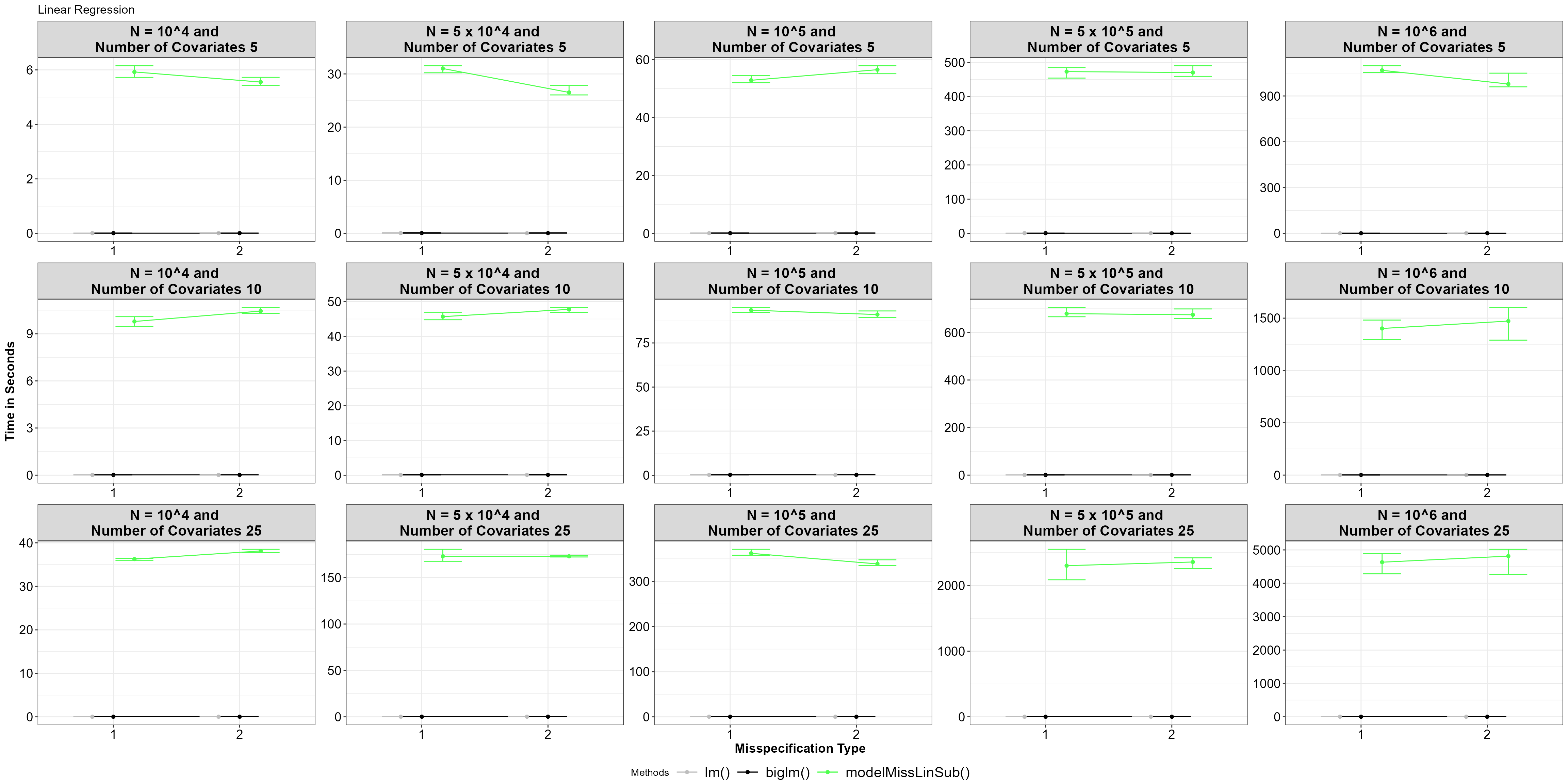
Average time for functions, with 5% and 95% percentile intervals under model misspecified linear regression.
In general, our subsampling functions perform slower as the size of the big data, the number of covariates, and the misspecification type differs. Calculating the reduction of loss value all data points is a significant bottleneck.
Logistic regression
For logistic regression, the modelMissLogSub() function
was compared against glm() and bigglm().
Functions_FCT<-c("glm()","bigglm()","modelMissLogSub()")
Functions_Colors<-c("cornsilk4","black","#50FF50")

Final_Logistic_Regression %>%
  mutate(Functions=factor(Functions,levels = Functions_FCT,labels = Functions_FCT),
         `N size`=factor(`N size`,levels = N_size,labels = N_size_labels),
         `N and Covariate size`=paste0("N = ",`N size`,
                                       " and \nNumber of Covariates ",
                                       `Covariate size`)) %>%
  mutate(`N and Covariate size`=factor(`N and Covariate size`,
                                       levels = N_and_CS_size,
                                       labels = N_and_CS_size)) %>%
  select(`N and Covariate size`,Misspecification,Functions,Time) %>%
  group_by(`N and Covariate size`,Misspecification,Functions) %>%
  summarise(Mean=mean(Time),min=quantile(Time,0.05),
            max=quantile(Time,0.95),.groups="drop") %>%
  ggplot(.,aes(x=factor(Misspecification),y=Mean,color=Functions,
               group=Functions))+
  geom_point(position = position_dodge(width = 0.5))+
  geom_line(position = position_dodge(width = 0.5))+
  geom_errorbar(aes(ymin=min,ymax=max),
                position = position_dodge(width = 0.5))+
  facet_wrap(.~factor(`N and Covariate size`),scales = "free",
             ncol=length(N_size))+
  xlab("Misspecification Type")+ylab("Time in Seconds")+
  scale_color_manual(values = Functions_Colors)+
  theme_bw()+Theme_special()+ggtitle("Logistic Regression")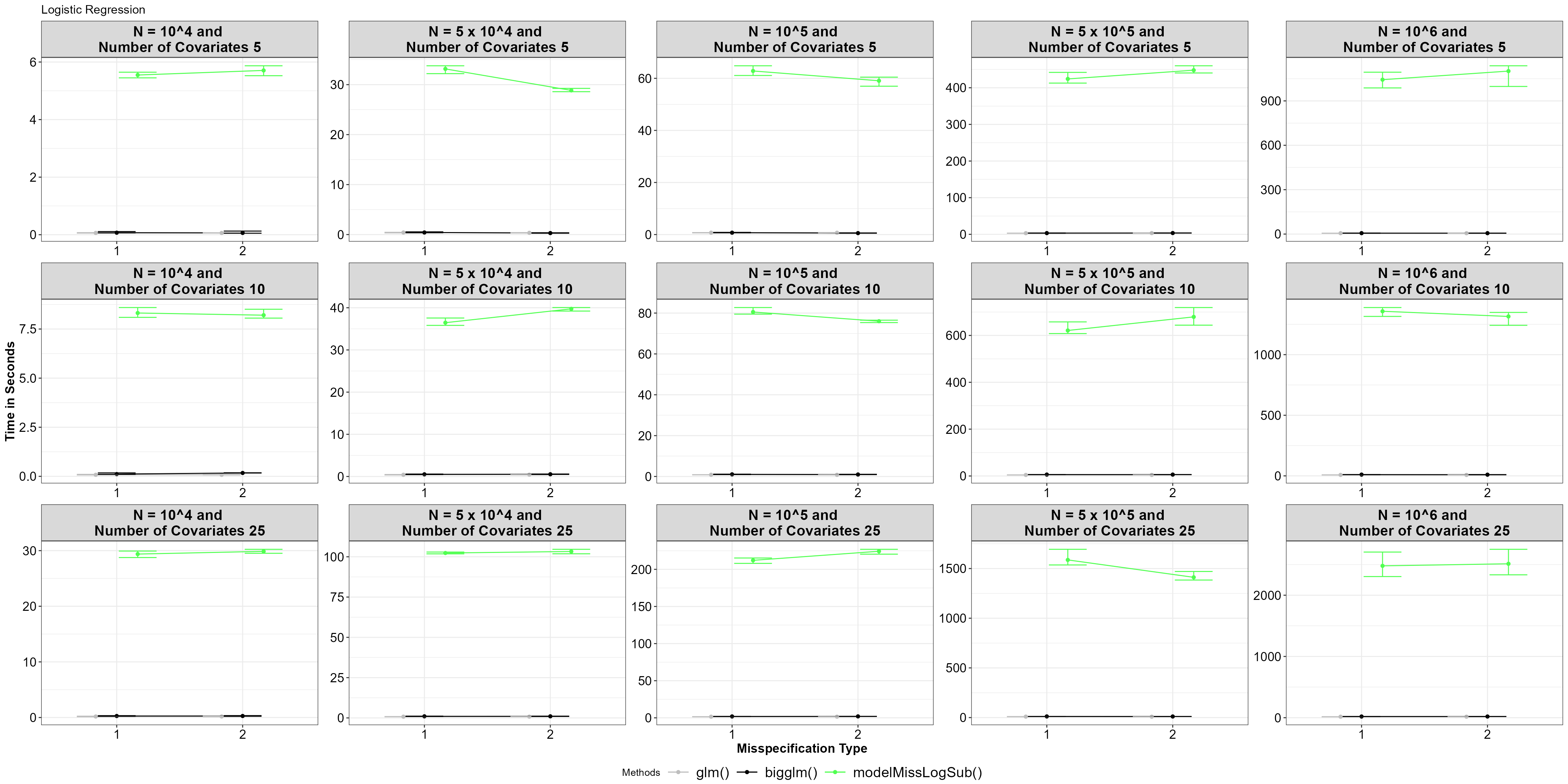
Average time for functions, with 5% and 95% percentile intervals under model misspecified logistic regression.
It seems there is a significant difference between using
glm() and bigglm(), with the
model-misspecified subsampling function performing slower. This
performance gap increases as the size of the big data and the number of
covariates grow irrespective of the misspecification type. As in model
misspecified subsampling under linear regression the bottleneck occurs
with calculating the reduction of loss for all data points of the big
data.
Poisson Regression
For Poisson regression, the function modelMissPoiSub()
was compared against glm() and bigglm().
Functions_FCT<-c("glm()","bigglm()","modelMissPoiSub()")
Functions_Colors<-c("cornsilk4","black","#50FF50")

Final_Poisson_Regression %>%
  mutate(Functions=factor(Functions,levels = Functions_FCT,labels = Functions_FCT),
         `N size`=factor(`N size`,levels = N_size,labels = N_size_labels),
         `N and Covariate size`=paste0("N = ",`N size`,
                                       " and \nNumber of Covariates ",
                                       `Covariate size`)) %>%
  mutate(`N and Covariate size`=factor(`N and Covariate size`,
                                       levels = N_and_CS_size,
                                       labels = N_and_CS_size)) %>%
  select(`N and Covariate size`,Misspecification,Functions,Time) %>%
  group_by(`N and Covariate size`,Misspecification,Functions) %>%
  summarise(Mean=mean(Time),min=quantile(Time,0.05),
            max=quantile(Time,0.95),.groups="drop") %>%
  ggplot(.,aes(x=factor(Misspecification),y=Mean,color=Functions,
               group=Functions))+
  geom_point(position = position_dodge(width = 0.5))+
  geom_line(position = position_dodge(width = 0.5))+
  geom_errorbar(aes(ymin=min,ymax=max),
                position = position_dodge(width = 0.5))+
  facet_wrap(.~factor(`N and Covariate size`),scales = "free",
             ncol=length(N_size))+
  xlab("Misspecification Type")+ylab("Time in Seconds")+
  scale_color_manual(values = Functions_Colors)+
  theme_bw()+Theme_special()+ggtitle("Poisson Regression")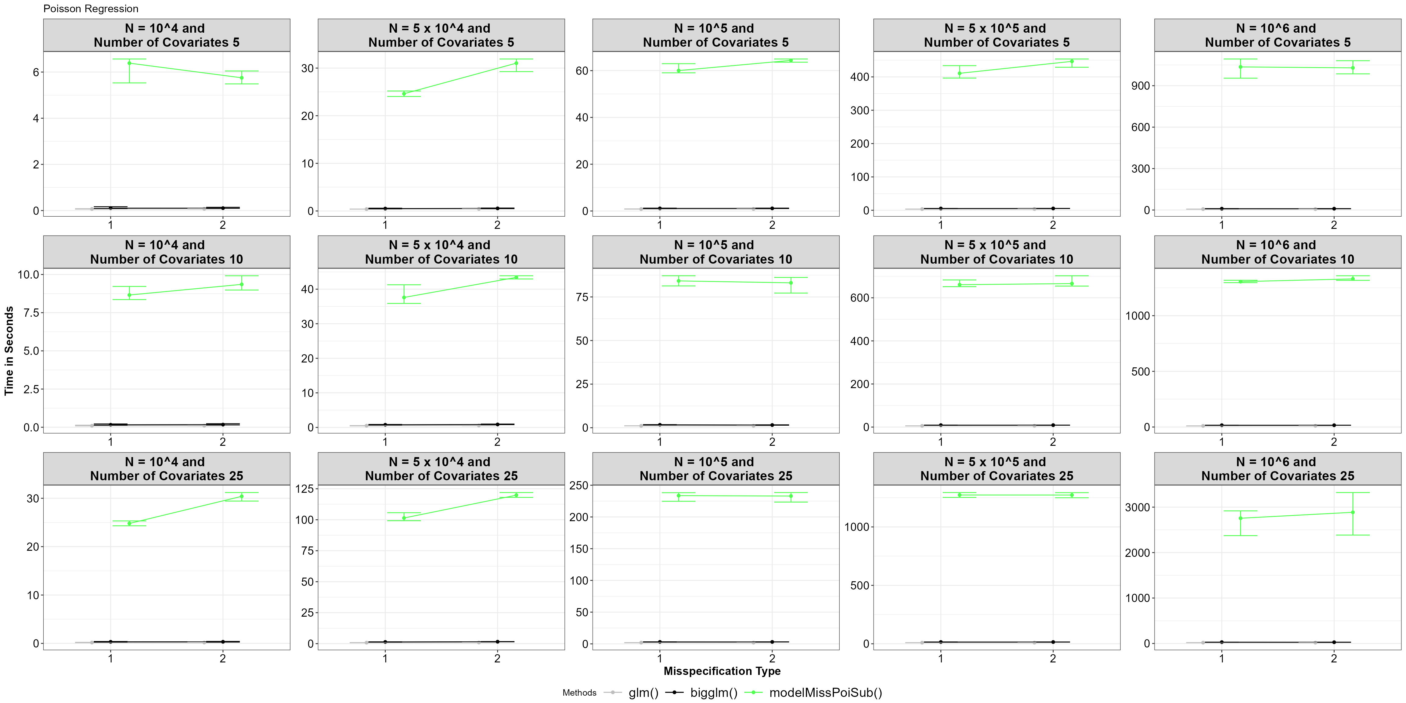
Average time for functions, with 5% and 95% percentile intervals under model misspecified Poisson regression.
Similar to logistic regression, the model misspecified subsampling
function performs slower than the glm() and
bigglm() functions.
In summary, the model misspecified subsampling functions available in this R package are limited in computation time as the reduction of loss is calculated for all data points. A potential solution would be to obtain this calculation for a proportion of the big data and continue the subsampling.