Benchmarking model-based subsampling functions
Source:vignettes/Benchmark_model_based.Rmd
Benchmark_model_based.Rmd## Error in get(paste0(generic, ".", class), envir = get_method_env()) :
## object 'type_sum.accel' not found
library(ggpubr)
library(tidyr)
library(dplyr)

# Theme for plots
Theme_special<-function(){
  theme(legend.key.width=unit(1,"cm"),
        axis.text.x = element_text(color = "black",size=14),
        axis.text.y = element_text(color = "black",size=14),
        strip.text = element_text(colour = "black",size = 16,face="bold"),
        panel.grid.minor.x = element_blank(),
        axis.title= element_text(color = "black",face = "bold",size = 14),
        legend.text = element_text(color = "black", size=16),
        legend.position = "bottom",
        legend.margin=margin(0,0,0,0),
        legend.box.margin=margin(-1,-2,-1,-2))
}

invisible(load("additionaldata/Results_Model_Based.Rdata"))
Setup
The lm(), biglm(), glm() and
bigglm() functions are benchmarked against the model-based
subsampling functions. Benchmarking is conducted across all three
regression problems using a consistent setup throughout. For the big
data sizes \(N = \{10^4,5 \times 10^4,10^5,5
\times 10^5,10^6,5 \times 10^6\}\) and for five different
Covariates sizes \(\{5,10,25,50,100\}\), the functions were
replicated \(100\) times. When using
the subsampling functions, the initial subsample sizes \(r_0=\{100,100,250,500,1000\}\) were
selected based on the covariate sizes, while the final subsample size
was fixed at \(r_f=2500\) to ensure
successful implementation.
N_size<-c(1,5,10,50,100,500)*10000
N_size_labels<-c("10^4","5 x 10^4","10^5","5 x 10^5","10^6","5 x 10^6")
CS_size<-c(5,10,25,50,100)
This implementation was conducted on a high-performance computing system; however, the code for linear regression-related functions is shown below. Furthermore, it can be extended to logistic and Poisson regression by incorporating the relevant subsampling functions and model configurations.
# load the packages
library(NeEDS4BigData)
library(here)
library(biglm)

# indexes for N and covariate sizes
indexA <- as.numeric(Sys.getenv("indexA"))
indexB <- as.numeric(Sys.getenv("indexB"))

# set N and covariate size, and assign replicates
N_size<-c(1,5,10,50,100,500)*10000
Covariate_size<-c(5,10,25,50,100)
Replicates<-50

# set the initial and final subsample sizes,
# with the distribution parameters to generate data
r0<-c(1,1,2.5,5,10)*100; rf<-2500;
Dist<-"Normal"; Dist_Par<-list(Mean=0,Variance=1,Error_Variance=0.5);
Family<-"linear"

# assign the indexes
N_idx<-indexA
Covariate_idx<-indexB
No_Of_Var<-Covariate_size[Covariate_idx]
N<-N_size[N_idx]

# generate the big data based on N and covariate size
Beta<-c(-1,rep(0.5,Covariate_size[Covariate_idx]))
Generated_Data<-GenGLMdata(Dist,Dist_Par,No_Of_Var,Beta,N,Family)
Full_Data<-Generated_Data$Complete_Data

cat("N size :",N_size[N_idx]," and Covariate size :",Covariate_size[Covariate_idx],"\n")

# formula for the linear regression model
lm_formula<-as.formula(paste("Y ~", paste(paste0("X",0:ncol(Full_Data[,-c(1,2)])),
                                          collapse = " + ")))

# benchmarking the stats::lm() function
lm<-sapply(1:Replicates,function(i){
  start_T<-Sys.time()
  suppressMessages(lm(Y~.-1,data=data.frame(Full_Data)))
  return(difftime(Sys.time(),start_T,units = "secs"))
})

cat("Benchmarked lm() function.\n")

# benchmarking the biglm::biglm() function
biglm<-sapply(1:Replicates,function(i){
  start_T<-Sys.time()
  suppressMessages(biglm(lm_formula,data=data.frame(Full_Data)))
  return(difftime(Sys.time(),start_T,units = "secs"))
})

cat("Benchmarked biglm() function.\n")

# benchmarking the NeEDS4BigData::AoptimalGauLMSub() function
AoptimalGauLMSub<-sapply(1:Replicates,function(i){
  start_T<-Sys.time()
  suppressMessages(AoptimalGauLMSub(r0[Covariate_idx],rf,
                                    Y=as.matrix(Full_Data[,1]),
                                    X=as.matrix(Full_Data[,-1]),
                                    N=nrow(Full_Data)))
  return(difftime(Sys.time(),start_T,units = "secs"))
})

cat("Benchmarked AoptimalGauLMSub() function.\n")

# benchmarking the NeEDS4BigData::LeverageSampling() function
LeverageSampling<-sapply(1:Replicates,function(i){
  start_T<-Sys.time()
  suppressMessages(LeverageSampling(rf,
                                    Y=as.matrix(Full_Data[,1]),
                                    X=as.matrix(Full_Data[,-1]),
                                    N=nrow(Full_Data),
                                    S_alpha=0.95,
                                    family=Family))
  return(difftime(Sys.time(),start_T,units = "secs"))
})

cat("Benchmarked LeverageSampling() function.\n")

# benchmarking the NeEDS4BigData::ALoptimalGLMSub() function
ALoptimalGLMSub<-sapply(1:Replicates,function(i){
  start_T<-Sys.time()
  suppressMessages(ALoptimalGLMSub(r0[Covariate_idx],rf,
                                   Y=as.matrix(Full_Data[,1]),
                                   X=as.matrix(Full_Data[,-1]),
                                   N=nrow(Full_Data),
                                   family=Family))
  return(difftime(Sys.time(),start_T,units = "secs"))
})

cat("Benchmarked ALoptimalGLMSub() function.\n")

# benchmarking the NeEDS4BigData::AoptimalMCGLMSub() function
AoptimalMCGLMSub<-sapply(1:Replicates,function(i){
  start_T<-Sys.time()
  suppressMessages(AoptimalMCGLMSub(r0[Covariate_idx],rf,
                                    Y=as.matrix(Full_Data[,1]),
                                    X=as.matrix(Full_Data[,-1]),
                                    N=nrow(Full_Data),
                                    family=Family))
  return(difftime(Sys.time(),start_T,units = "secs"))
})

cat("Benchmarked AoptimalMCGLMSub() function.\n")

Plot_Data<-cbind.data.frame("N size"=N_size[N_idx],
                            "Covariate size"=Covariate_size[Covariate_idx],"lm()"=lm,
                            "biglm()"=biglm,"AoptimalGauLMSub()"=AoptimalGauLMSub,
                            "LeverageSampling()"=LeverageSampling,
                            "ALoptimalGLMSub()"=ALoptimalGLMSub,
                            "AoptimalMCGLMSub()"=AoptimalMCGLMSub)

save(Plot_Data,
     file=here("Results",paste0("Output_NS_",N_idx,"_CS_",Covariate_idx,".RData")))
Linear Regression
For linear regression, the following functions from the NeEDS4BigData
package: (1) AoptimalGauLMSub(), (2)
LeverageSampling(), (3) ALoptimalGLMSub(), and
(4) AoptimalMCGLMSub() are compared against
lm() and biglm().
Functions_FCT<-c("lm()","biglm()","LeverageSampling()","AoptimalMCGLMSub()",
               "AoptimalGauLMSub()","ALoptimalGLMSub()")
Functions_Colors<-c("cornsilk4","black","#F76D5E","#A50021","#BBFFBB","#50FF50")

Final_Linear_Regression %>%
  group_by(`N size`,`Covariate size`,Functions) %>%
  summarise(Mean=mean(Time),min=quantile(Time,0.05),max=quantile(Time,0.95),
            .groups = "drop") %>%
  mutate(Functions=factor(Functions,levels = Functions_FCT,labels = Functions_FCT),
         `N size`=factor(`N size`,levels = N_size,
                         labels=paste0("N = ",N_size_labels))) %>%
ggplot(.,aes(x=factor(`Covariate size`),y=Mean,color=Functions,group=Functions))+
  geom_point(position = position_dodge(width = 0.5))+
  geom_line(position = position_dodge(width = 0.5))+
  geom_errorbar(aes(ymin=min,ymax=max),position = position_dodge(width = 0.5))+
  facet_wrap(~factor(`N size`),scales = "free",nrow=2)+
  xlab("Number of Covariates")+ylab("Time in Seconds")+
  scale_color_manual(values = Functions_Colors)+
  theme_bw()+ggtitle("Linear Regression")+Theme_special()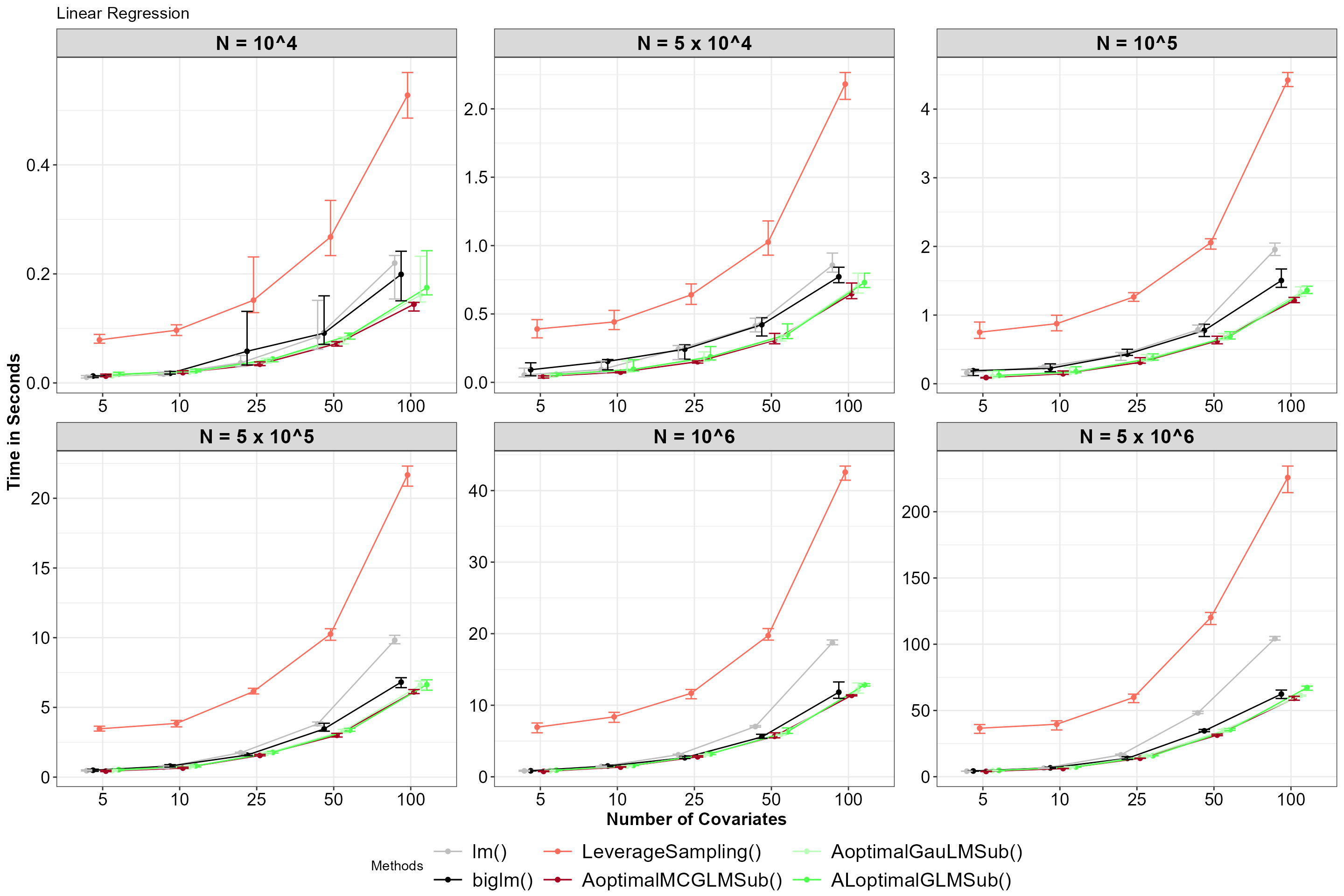
Average time for functions, with 5% and 95% percentile intervals under linear regression.
In general, our subsampling functions perform faster as the size of
the big data and the number of covariates increase, except for
LeverageSampling(). Even when a solution for linear
regression is available in an analytical form, the subsampling functions
perform as well as biglm().
Logistic Regression
For logistic regression, the following functions: (1)
LCCSampling(), (2) LeverageSampling(), (3)
AoptimalMCGLMSub(), and (4) ALoptimalGLMSub()
are compared against glm() and bigglm().
Functions_FCT<-c("glm()","bigglm()","LCCSampling()","LeverageSampling()",
               "AoptimalMCGLMSub()","ALoptimalGLMSub()")
Functions_Colors<-c("cornsilk4","black","#F76D5E","#A50021","#BBFFBB","#50FF50")

Final_Logistic_Regression %>%
  group_by(`N size`,`Covariate size`,Functions) %>%
  summarise(Mean=mean(Time),min=quantile(Time,0.05),max=quantile(Time,0.95),
            .groups = "drop") %>%
  mutate(Functions=factor(Functions,levels = Functions_FCT,labels = Functions_FCT),
         `N size`=factor(`N size`,levels = N_size,
                         labels=paste0("N = ",N_size_labels))) %>%
ggplot(.,aes(x=factor(`Covariate size`),y=Mean,color=Functions,group=Functions))+
  geom_point(position = position_dodge(width = 0.5))+
  geom_line(position = position_dodge(width = 0.5))+
  geom_errorbar(aes(ymin=min,ymax=max),position = position_dodge(width = 0.5))+
  facet_wrap(~factor(`N size`),scales = "free",nrow=2)+
  xlab("Number of Covariates")+ylab("Time in Seconds")+
  scale_color_manual(values = Functions_Colors)+
  theme_bw()+Theme_special()+ggtitle("Logistic Regression")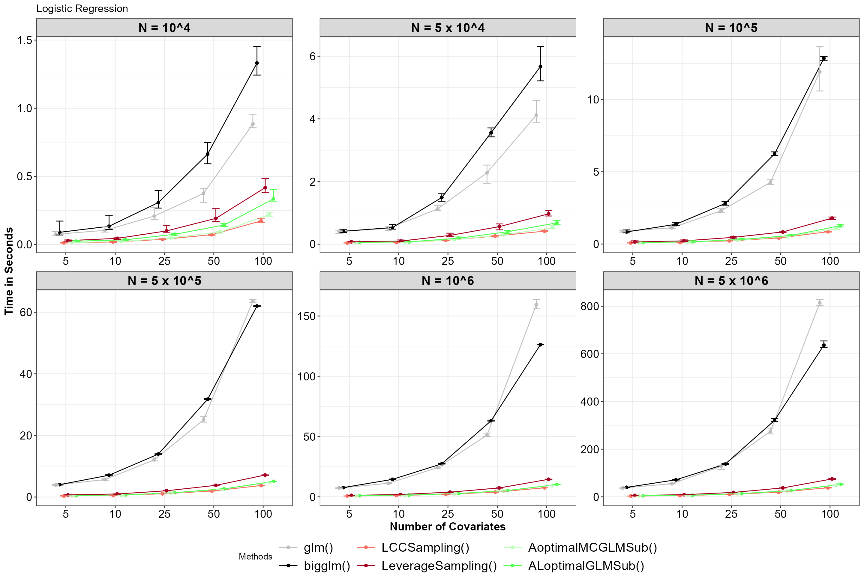
Average time for functions, with 5% and 95% percentile intervals under logistic regression.
There seems to be little difference between using glm()
and bigglm(), while the subsampling functions perform
faster, with the performance gap increasing as the size of the big data
and the number of covariates grow.
Poisson Regression
For Poisson regression, the following functions: (1)
LeverageSampling(), (2) AoptimalMCGLMSub(),
and (3) ALoptimalGLMSub() are compared against
glm() and bigglm().
Functions_FCT<-c("glm()","bigglm()","LeverageSampling()",
               "AoptimalMCGLMSub()","ALoptimalGLMSub()")
Functions_Colors<-c("cornsilk4","black","#A50021","#BBFFBB","#50FF50")

Final_Poisson_Regression %>%
  group_by(`N size`,`Covariate size`,Functions) %>%
  summarise(Mean=mean(Time),min=quantile(Time,0.05),max=quantile(Time,0.95),
            .groups = "drop") %>%
  mutate(Functions=factor(Functions,levels = Functions_FCT,labels = Functions_FCT),
         `N size`=factor(`N size`,levels = N_size,
                         labels=paste0("N = ",N_size_labels))) %>%
ggplot(.,aes(x=factor(`Covariate size`),y=Mean,color=Functions,group=Functions))+
  geom_point(position = position_dodge(width = 0.5))+
  geom_line(position = position_dodge(width = 0.5))+
  geom_errorbar(aes(ymin=min,ymax=max),position = position_dodge(width = 0.5))+
  facet_wrap(~factor(`N size`),scales = "free",nrow=2)+
  xlab("Number of Covariates")+ylab("Time in Seconds")+
  scale_color_manual(values = Functions_Colors)+
  theme_bw()+Theme_special()+ggtitle("Poisson Regression")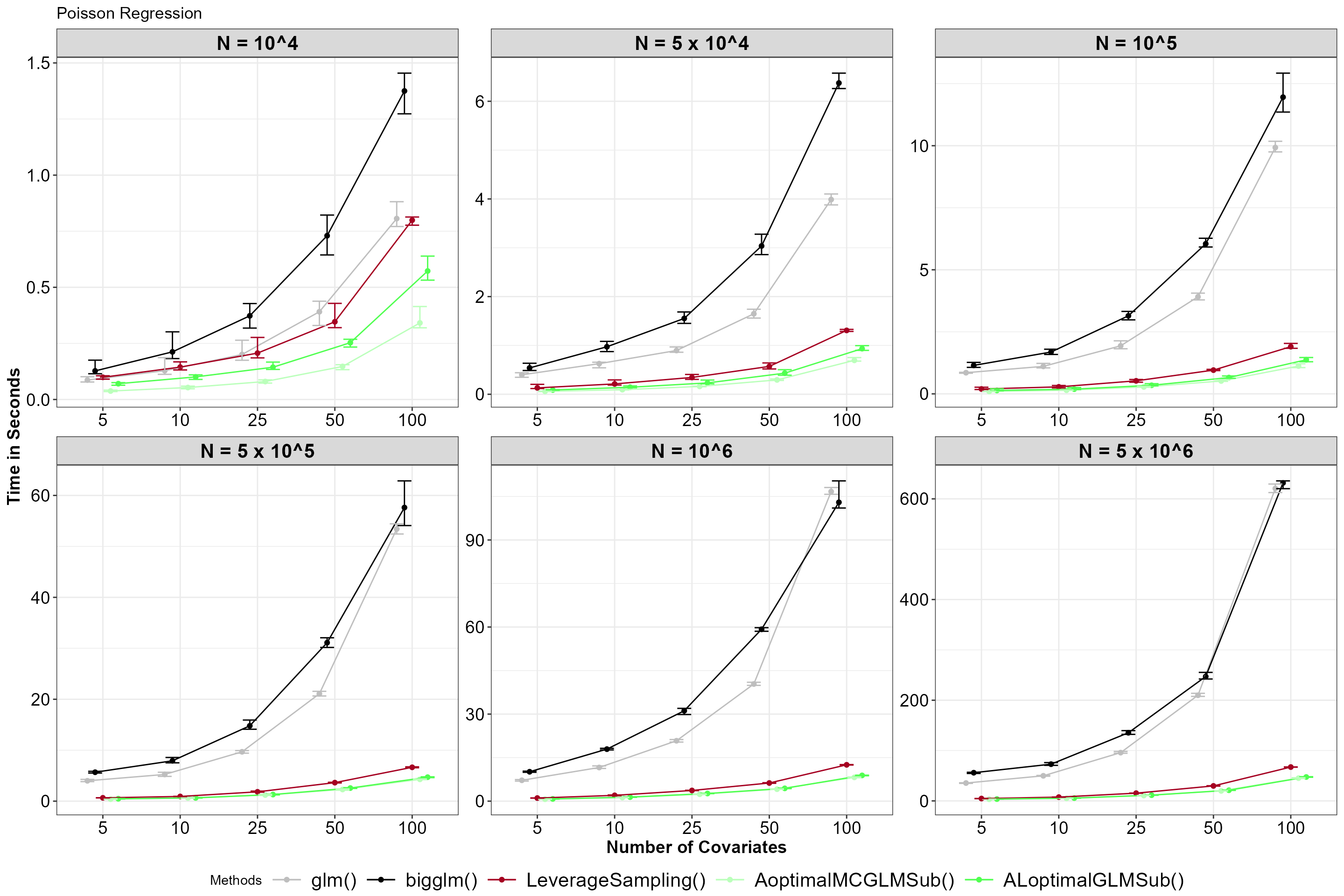
Average time for functions, with 5% and 95% percentile intervals under Poisson regression.
Similar to logistic regression, the subsampling functions perform
faster than the glm() and bigglm()
functions.
In summary, the subsampling functions available in this R package perform best under high-dimensional data.