A-optimality criteria based subsampling under measurement constraints for Generalised Linear Models
Source:R/AoptimalMCGLMSub.R
AoptimalMCGLMSub.RdUsing this function sample from big data under linear, logistic and Poisson regression to describe the data when response \(y\) is partially unavailable. Subsampling probabilities are obtained based on the A-optimality criteria.
Arguments
- r0
sample size for initial random sample
- rf
final sample size including initial(r0) and optimal(r) samples
- Y
response data or Y
- X
covariate data or X matrix that has all the covariates (first column is for the intercept)
- N
size of the big data
- family
a character value for "linear", "logistic" and "poisson" regression from Generalised Linear Models
Value
The output of AoptimalMCGLMSub gives a list of
Beta_Estimates estimated model parameters in a data.frame after subsampling
Variance_Epsilon_Estimates matrix of estimated variance for epsilon in a data.frame after subsampling (valid only for linear regression)
Sample_A-Optimality list of indexes for the initial and optimal samples obtained based on A-Optimality criteria
Subsampling_Probability matrix of calculated subsampling probabilities for A-optimality criteria
Details
Two stage subsampling algorithm for big data under Generalised Linear Models (linear, logistic and Poisson regression) when the response is not available for subsampling probability evaluation.
First stage is to obtain a random sample of size \(r_0\) and estimate the model parameters. Using the estimated parameters subsampling probabilities are evaluated for A-optimality criteria.
Through the estimated subsampling probabilities an optimal sample of size \(r \ge r_0\) is obtained. Finally, only the optimal sample is used and the model parameters are estimated.
NOTE : If input parameters are not in given domain conditions necessary error messages will be provided to go further.
If \(r \ge r_0\) is not satisfied then an error message will be produced.
If the big data \(X,Y\) has any missing values then an error message will be produced.
The big data size \(N\) is compared with the sizes of \(X,Y\) and if they are not aligned an error message will be produced.
A character value is provided for family and if it is not of the any three types an error message
will be produced.
References
Zhang T, Ning Y, Ruppert D (2021). “Optimal sampling for generalized linear models under measurement constraints.” Journal of Computational and Graphical Statistics, 30(1), 106--114.
Examples
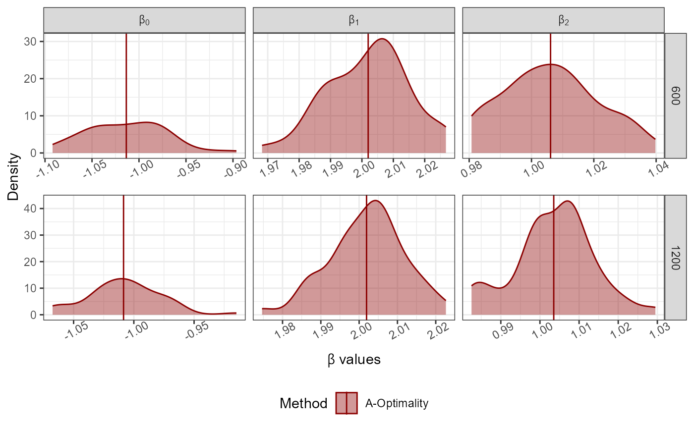
Dist<-"Normal"; Dist_Par<-list(Mean=0,Variance=1,Error_Variance=0.5)
No_Of_Var<-2; Beta<-c(-1,2,1); N<-10000; Family<-"linear"
Full_Data<-GenGLMdata(Dist,Dist_Par,No_Of_Var,Beta,N,Family)
r0<-300; rf<-rep(100*c(6,12),50); Original_Data<-Full_Data$Complete_Data;
AoptimalMCGLMSub(r0 = r0, rf = rf,Y = as.matrix(Original_Data[,1]),
X = as.matrix(Original_Data[,-1]),N = nrow(Original_Data),
family = "linear")->Results
#> Step 1 of the algorithm completed.
#> Step 2 of the algorithm completed.
plot_Beta(Results)
#> Picking joint bandwidth of 0.00889
#> Picking joint bandwidth of 0.00923
#> Picking joint bandwidth of 0.00796
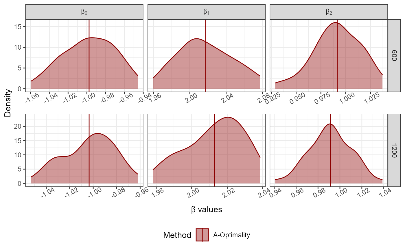 Dist<-"Normal"; Dist_Par<-list(Mean=0,Variance=1)
No_Of_Var<-2; Beta<-c(-1,2,1); N<-10000; Family<-"logistic"
Full_Data<-GenGLMdata(Dist,Dist_Par,No_Of_Var,Beta,N,Family)
r0<-300; rf<-rep(100*c(6,12),50); Original_Data<-Full_Data$Complete_Data;
AoptimalMCGLMSub(r0 = r0, rf = rf,Y = as.matrix(Original_Data[,1]),
X = as.matrix(Original_Data[,-1]),N = nrow(Original_Data),
family = "logistic")->Results
#> Step 1 of the algorithm completed.
#> Step 2 of the algorithm completed.
plot_Beta(Results)
#> Picking joint bandwidth of 0.0494
#> Picking joint bandwidth of 0.0636
#> Picking joint bandwidth of 0.0375
Dist<-"Normal"; Dist_Par<-list(Mean=0,Variance=1)
No_Of_Var<-2; Beta<-c(-1,2,1); N<-10000; Family<-"logistic"
Full_Data<-GenGLMdata(Dist,Dist_Par,No_Of_Var,Beta,N,Family)
r0<-300; rf<-rep(100*c(6,12),50); Original_Data<-Full_Data$Complete_Data;
AoptimalMCGLMSub(r0 = r0, rf = rf,Y = as.matrix(Original_Data[,1]),
X = as.matrix(Original_Data[,-1]),N = nrow(Original_Data),
family = "logistic")->Results
#> Step 1 of the algorithm completed.
#> Step 2 of the algorithm completed.
plot_Beta(Results)
#> Picking joint bandwidth of 0.0494
#> Picking joint bandwidth of 0.0636
#> Picking joint bandwidth of 0.0375
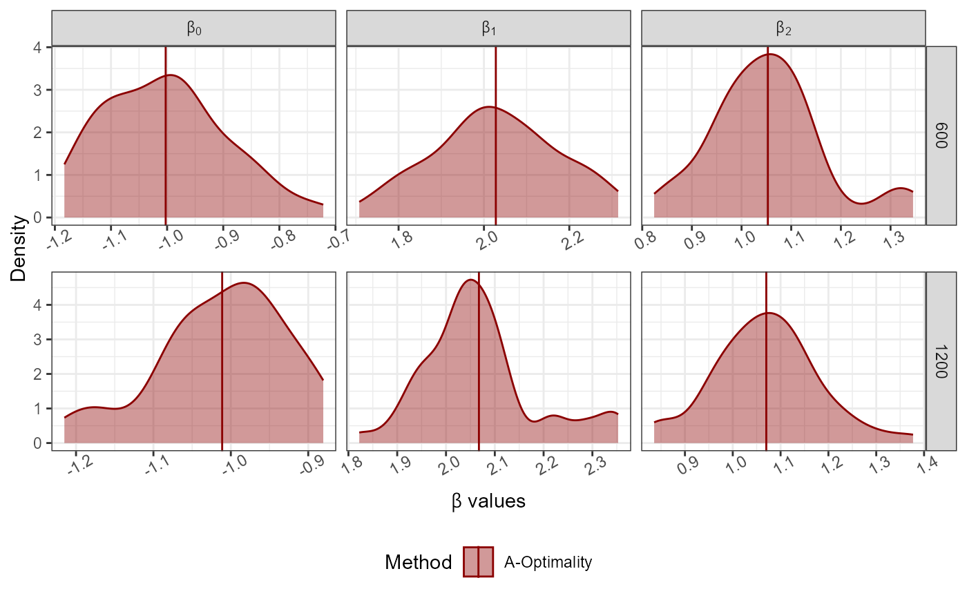 Dist<-"Normal";
No_Of_Var<-2; Beta<-c(-1,2,1); N<-10000; Family<-"poisson"
Full_Data<-GenGLMdata(Dist,NULL,No_Of_Var,Beta,N,Family)
r0<-300; rf<-rep(100*c(6,12),50); Original_Data<-Full_Data$Complete_Data;
AoptimalMCGLMSub(r0 = r0, rf = rf,Y = as.matrix(Original_Data[,1]),
X = as.matrix(Original_Data[,-1]),N = nrow(Original_Data),
family = "poisson")->Results
#> Step 1 of the algorithm completed.
#> Step 2 of the algorithm completed.
plot_Beta(Results)
#> Picking joint bandwidth of 0.0142
#> Picking joint bandwidth of 0.00581
#> Picking joint bandwidth of 0.00479
Dist<-"Normal";
No_Of_Var<-2; Beta<-c(-1,2,1); N<-10000; Family<-"poisson"
Full_Data<-GenGLMdata(Dist,NULL,No_Of_Var,Beta,N,Family)
r0<-300; rf<-rep(100*c(6,12),50); Original_Data<-Full_Data$Complete_Data;
AoptimalMCGLMSub(r0 = r0, rf = rf,Y = as.matrix(Original_Data[,1]),
X = as.matrix(Original_Data[,-1]),N = nrow(Original_Data),
family = "poisson")->Results
#> Step 1 of the algorithm completed.
#> Step 2 of the algorithm completed.
plot_Beta(Results)
#> Picking joint bandwidth of 0.0142
#> Picking joint bandwidth of 0.00581
#> Picking joint bandwidth of 0.00479