Model based Sampling for Logistic Regression
Source:vignettes/Basic_Sampling_Log_Reg.Rmd
Basic_Sampling_Log_Reg.Rmd
# Load the R packages
library(NeEDS4BigData)
library(ggplot2)
library(ggpubr)
library(kableExtra)
library(tidyr)
library(psych)
library(gam)

# Theme for plots
Theme_special<-function(){
  theme(legend.key.width= unit(1,"cm"),
        axis.text.x= element_text(color= "black", size= 12, angle= 30, hjust=0.75),
        axis.text.y= element_text(color= "black", size= 12),
        strip.text= element_text(colour= "black", size= 12, face= "bold"),
        panel.grid.minor.x= element_blank(),
        axis.title= element_text(color= "black", face= "bold", size= 12),
        legend.text= element_text(color= "black", size= 11),
        legend.position= "bottom",
        legend.margin= margin(0,0,0,0),
        legend.box.margin= margin(-1,-2,-1,-2))
}
Understanding the skin segmentation data
Rajen and Abhinav (2012) addressed the challenge of detecting skin-like regions in images as a component of the intricate process of facial recognition. To achieve this goal, the ``Skin segmentation data’’ was curated, this data contains \(4\) columns and has \(245,057\) observations, first column is the response variable and the rest are covariates. Aim of the logistic regression model is to classify if images are skin or not based on the a) Red, b) Green and c) Blue colour data. Skin presence is denoted as one and skin absence is denoted as zero. Each colour vector is scaled to have a mean of zero and a variance of one (initial range was between 0−255). For the given data sampling methods are implemented assuming the main effects model can describe the data.
# Selecting 100% of the big data and prepare it
indexes<-1:nrow(Skin_segmentation)
Original_Data<-cbind(Skin_segmentation[indexes,1],1,Skin_segmentation[indexes,-1])
colnames(Original_Data)<-c("Y",paste0("X",0:ncol(Original_Data[,-c(1,2)])))

# Scaling the covariate data
for (j in 3:5) {
  Original_Data[,j]<-scale(Original_Data[,j])
}
head(Original_Data) %>%
  kable(format = "html",
caption = "First few observations of the skin segmentation data.")| Y | X0 | X1 | X2 | X3 |
|---|---|---|---|---|
| 0 | 1 | -0.8202540 | -0.7925655 | -0.002441364 |
| 0 | 1 | -0.8363168 | -0.8092485 | -0.016222650 |
| 0 | 1 | -0.8523796 | -0.8259316 | -0.030003937 |
| 0 | 1 | -0.8845052 | -0.8592976 | -0.057566510 |
| 0 | 1 | -0.8845052 | -0.8592976 | -0.057566510 |
| 0 | 1 | -0.9005680 | -0.8759806 | -0.071347797 |
# Setting the sample sizes
N<-nrow(Original_Data); M<-250; k<-seq(6,18,by=3)*100; rep_k<-rep(k,each=M)
Based on this model the methods random sampling, leverage sampling (Ma, Mahoney, and Yu 2014; Ma and Sun 2015), local case control sampling (Fithian and Hastie 2015), \(A\)- and \(L\)-optimality subsampling (Ai et al. 2021; Yao and Wang 2021) and \(A\)-optimality sampling with response constraint (Zhang, Ning, and Ruppert 2021) are implemented on the big data.
# define colours, shapes, line types for the methods
Method_Names<-c("A-Optimality","L-Optimality","A-Optimality MC",
                "Local case control sampling","Shrinkage Leverage",
                "Basic Leverage","Unweighted Leverage","Random sampling")
Method_Colour<-c("green","green4","yellowgreen",
                 "maroon","red","darkred","firebrick","black")
Method_Shape_Types<-c(rep(8,3),rep(4,4),16)
Method_Line_Types<-c(rep("twodash",3),rep("dotted",4),"solid")
The obtained samples and their respective model parameter estimates are over \(M=100\) simulations across different sample sizes \(k=(600,\ldots,1500)\). We set the initial sample size of \(r1=300\) for the methods that requires a random sample. From the final samples, model parameters of the assume model are estimated. These estimated model parameters are compared with the estimated model parameters of the full big data through the mean squared error \(MSE(\tilde{\beta}_k,\hat{\beta})=\frac{1}{MJ}\sum_{i=1}^M \sum_{j=1}^J(\tilde{\beta}_{k,j} - \hat{\beta}_j)^2\). Here, \(\tilde{\beta}_k\) is the estimated model parameters from the sample of size \(k\) and \(\hat{\beta}\) is the estimated model parameters from the full big data, while \(j\) is index of the model parameter.
Random sampling
Below is the code for this implementation.
# Random sampling
Final_Beta_RS<-matrix(nrow = length(k)*M,ncol = ncol(Original_Data[,-1])+1)
for (i in 1:length(rep_k)) {
  Temp_Data<-Original_Data[sample(1:N,rep_k[i]),]
  glm(Y~.-1,data=Temp_Data,family="binomial")->Results
  Final_Beta_RS[i,]<-c(rep_k[i],coefficients(Results))
  if(i==length(rep_k)){print("All simulations completed for random sampling")}
}
## [1] "All simulations completed for random sampling"
Final_Beta_RS<-cbind.data.frame("Random sampling",Final_Beta_RS)
colnames(Final_Beta_RS)<-c("Method","Sample",paste0("Beta",0:3))
Leverage sampling
# Leverage sampling
## we set the shrinkage value of alpha=0.9
NeEDS4BigData::LeverageSampling(r=rep_k,Y=as.matrix(Original_Data[,1]),
                                X=as.matrix(Original_Data[,-1]),N=N,
                                alpha = 0.9,family = "logistic")->Results
## Basic and shrinkage leverage probabilities calculated.## Sampling completed.Local case control sampling
# Local case control sampling
NeEDS4BigData::LCCsampling(r1=300,r2=rep_k,
                           Y=as.matrix(Original_Data[,1]),
                           X=as.matrix(Original_Data[,-1]),
                           N=N)->Results
## Step 1 of the algorithm completed.## Step 2 of the algorithm completed.A- and L-optimality subsampling
# A- and L-optimality subsampling for GLM
NeEDS4BigData::ALoptimalGLMSub(r1=300,r2=rep_k,
                               Y=as.matrix(Original_Data[,1]),
                               X=as.matrix(Original_Data[,-1]),
                               N=N,family = "logistic")->Results
## Step 1 of the algorithm completed.## Step 2 of the algorithm completed.A-optimality sampling under measurement constraints
# A-optimality sampling for without response
NeEDS4BigData::AoptimalMCGLMSub(r1=300,r2=rep_k,
                                Y=as.matrix(Original_Data[,1]),
                                X=as.matrix(Original_Data[,-1]),
                                N=N,family="logistic")->Results
## Step 1 of the algorithm completed.## Step 2 of the algorithm completed.Summary
# Summarising Results of Scenario one
Final_Beta<-rbind(Final_Beta_RS,Final_Beta_LS,Final_Beta_LCCS,
                  Final_Beta_ALoptGLM,Final_Beta_AoptMCGLM)

# Obtaining the model parameter estimates for the full big data model
glm(Y~.-1,data = Original_Data,family="binomial")->All_Results
coefficients(All_Results)->All_Beta
matrix(rep(All_Beta,by=nrow(Final_Beta)),nrow = nrow(Final_Beta),
       ncol = ncol(Final_Beta[,-c(1,2)]),byrow = TRUE)->All_Beta

remove(Final_Beta_RS,Final_Beta_LS,Final_Beta_LCCS,Final_Beta_ALoptGLM,
       Final_Beta_AoptMCGLM,Temp_Data,Results,All_Results)
The mean squared error is plotted below.
# Obtain the mean squared error for the model parameter estimates
MSE_Beta<-data.frame("Method"=Final_Beta$Method,
                     "Sample"=Final_Beta$Sample,
                     "MSE"=rowSums((All_Beta - Final_Beta[,-c(1,2)])^2))

MSE_Beta$Method<-factor(MSE_Beta$Method,levels = Method_Names,labels = Method_Names)

# Plot for the mean squared error with all methods
ggplot(MSE_Beta |> dplyr::group_by(Method,Sample) |>
       dplyr::summarise(MSE=mean(MSE), .groups = 'drop'),
    aes(x=factor(Sample),y=MSE,color=Method,group=Method,
        linetype=Method,shape=Method))+
  geom_point()+geom_line()+xlab("Sample size")+ylab("MSE")+
  scale_color_manual(values = Method_Colour)+
  scale_linetype_manual(values=Method_Line_Types)+
  scale_shape_manual(values = Method_Shape_Types)+
  theme_bw()+guides(colour = guide_legend(nrow = 3))+Theme_special()->p1

# Plot for the mean squared error with all methods except unweighted leverage
ggplot(MSE_Beta[!(MSE_Beta$Method %in% c("Unweighted Leverage","Shrinkage Leverage",
                                         "Basic Leverage")),] |>
       dplyr::group_by(Method,Sample) |>
       dplyr::summarise(MSE=mean(MSE),.groups = 'drop'),
    aes(x=factor(Sample),y=MSE,color=Method,group=Method,
        linetype=Method,shape=Method))+
  geom_point()+geom_line()+xlab("Sample size")+ylab("MSE")+
  scale_color_manual(values = Method_Colour[-7])+
  scale_linetype_manual(values=Method_Line_Types[-7])+
  scale_shape_manual(values = Method_Shape_Types[-7])+
  theme_bw()+guides(colour = guide_legend(nrow = 3))+Theme_special()->p2

ggarrange(p1,p2,nrow = 2,ncol = 1,labels = "auto")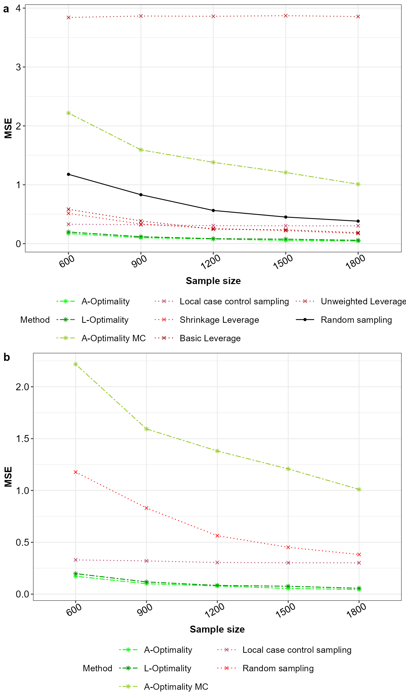
Mean squared error for a) all the sampling methods and b) without unweighted leverage sampling.