Model based Sampling for Linear Regression
Source:vignettes/Basic_Sampling_Lin_Reg.Rmd
Basic_Sampling_Lin_Reg.Rmd
# Load the R packages
library(NeEDS4BigData)
library(ggplot2)
library(ggpubr)
library(kableExtra)
library(tidyr)
library(psych)
library(gam)

# Theme for plots
Theme_special<-function(){
  theme(legend.key.width= unit(1,"cm"),
        axis.text.x= element_text(color= "black", size= 12, angle= 30, hjust=0.75),
        axis.text.y= element_text(color= "black", size= 12),
        strip.text= element_text(colour= "black", size= 12, face= "bold"),
        panel.grid.minor.x= element_blank(),
        axis.title= element_text(color= "black", face= "bold", size= 12),
        legend.text= element_text(color= "black", size= 11),
        legend.position= "bottom",
        legend.margin= margin(0,0,0,0),
        legend.box.margin= margin(-1,-2,-1,-2))
}
Understanding the electric consumption data
``Electric power consumption’’ data (Hebrail and Berard 2012), which contains \(2,049,280\) measurements for a house located at Sceaux, France between December 2006 and November 2010. The data contains \(4\) columns, the first column is the response variable and the rest are covariates, however we only use the first \(5\%\) of the data for this demonstration. The response \(y\) is the log scaled intensity, while the covariates are active electrical energy in the a) kitchen (\(X_1\)), b) laundry room (\(X_2\)) and c) water-heater and air-conditioner (\(X_3\)). The covariates are scaled to be mean of zero and variance of one. For the given data sampling methods are implemented assuming the main effects model can describe the data.
# Selecting 5% of the big data and prepare it
indexes<-1:ceiling(nrow(Electric_consumption)*0.05)
Original_Data<-cbind(Electric_consumption[indexes,1],1,Electric_consumption[indexes,-1])
colnames(Original_Data)<-c("Y",paste0("X",0:ncol(Original_Data[,-c(1,2)])))

# Scaling the covariate data
for (j in 3:5) {
  Original_Data[,j]<-scale(Original_Data[,j])
}
head(Original_Data) %>%
  kable(format = "html",
caption = "First few observations of the electric consumption data.")| Y | X0 | X1 | X2 | X3 |
|---|---|---|---|---|
| 2.912351 | 1 | -0.1941391 | -0.11558111 | 1.112635 |
| 3.135494 | 1 | -0.1941391 | -0.11558111 | 0.996989 |
| 3.135494 | 1 | -0.1941391 | 0.01734184 | 1.112635 |
| 3.135494 | 1 | -0.1941391 | -0.11558111 | 1.112635 |
| 2.760010 | 1 | -0.1941391 | -0.11558111 | 1.112635 |
| 2.708050 | 1 | -0.1941391 | 0.01734184 | 1.112635 |
# Setting the sample sizes
N<-nrow(Original_Data); M<-250; k<-seq(6,18,by=3)*100; rep_k<-rep(k,each=M)
Based on this model the methods random sampling, leverage sampling (Ma, Mahoney, and Yu 2014; Ma and Sun 2015), \(A\)-optimality sampling with Gaussian Linear Model (Lee, Schifano, and Wang 2022), \(A\)- and \(L\)-optimality subsampling (Ai et al. 2021; Yao and Wang 2021) and \(A\)-optimality sampling with response constraint (Zhang, Ning, and Ruppert 2021) are implemented on the big data.
# define colours, shapes, line types for the methods
Method_Names<-c("A-Optimality","L-Optimality","A-Optimality GauLM","A-Optimality MC",
                "Shrinkage Leverage","Basic Leverage","Unweighted Leverage",
                "Random Sampling")
Method_Colour<-c("yellowgreen","green4","green","springgreen4",
                 "red","darkred","maroon","black")
Method_Shape_Types<-c(rep(8,4),rep(4,3),16)
Method_Line_Types<-c(rep("twodash",4),rep("dotted",3),"solid")
The obtained samples and their respective model parameter estimates are over \(M=100\) simulations across different sample sizes \(k=(600,\ldots,1500)\). We set the initial sample size of \(r1=300\) for the methods that requires a random sample. From the final samples, model parameters of the assume model are estimated. These estimated model parameters are compared with the estimated model parameters of the full big data through the mean squared error \(MSE(\tilde{\beta}_k,\hat{\beta})=\frac{1}{MJ}\sum_{i=1}^M \sum_{j=1}^J(\tilde{\beta}_{k,j} - \hat{\beta}_j)^2\). Here, \(\tilde{\beta}_k\) is the estimated model parameters from the sample of size \(k\) and \(\hat{\beta}\) is the estimated model parameters from the full big data, while \(j\) is index of the model parameter.
Random sampling
Below is the code for implementing these sampling methods.
# Random sampling
Final_Beta_RS<-matrix(nrow = length(k)*M,ncol = ncol(Original_Data[,-1])+1)
for (i in 1:length(rep_k)) {
  Temp_Data<-Original_Data[sample(1:N,rep_k[i]),]
  lm(Y~.-1,data=Temp_Data)->Results
  Final_Beta_RS[i,]<-c(rep_k[i],coefficients(Results))
  if(i==length(rep_k)){print("All simulations completed for random sampling")}
}
## [1] "All simulations completed for random sampling"
Final_Beta_RS<-cbind.data.frame("Random Sampling",Final_Beta_RS)
colnames(Final_Beta_RS)<-c("Method","Sample",paste0("Beta",0:3))
Leverage sampling
# Leverage sampling
## we set the shrinkage value of alpha=0.9
NeEDS4BigData::LeverageSampling(r=rep_k,Y=as.matrix(Original_Data[,1]),
                                X=as.matrix(Original_Data[,-1]),N=N,
                                alpha = 0.9,family = "linear")->Results
## Basic and shrinkage leverage probabilities calculated.## Sampling completed.A-optimality subsampling for Gaussian Linear Model
# A-optimality subsampling for Gaussian Linear Model
NeEDS4BigData::AoptimalGauLMSub(r1=300,r2=rep_k,
                                Y=as.matrix(Original_Data[,1]),
                                X=as.matrix(Original_Data[,-1]),N=N)->Results
## Step 1 of the algorithm completed.## Step 2 of the algorithm completed.A- and L-optimality subsampling
# A- and L-optimality subsampling for GLM
NeEDS4BigData::ALoptimalGLMSub(r1=300,r2=rep_k,
                               Y=as.matrix(Original_Data[,1]),
                               X=as.matrix(Original_Data[,-1]),
                               N=N,family = "linear")->Results
## Step 1 of the algorithm completed.## Step 2 of the algorithm completed.A-optimality sampling with measurement constraints
# A-optimality sampling for without response
NeEDS4BigData::AoptimalMCGLMSub(r1=300,r2=rep_k,
                                Y=as.matrix(Original_Data[,1]),
                                X=as.matrix(Original_Data[,-1]),
                                N=N,family="linear")->Results
## Step 1 of the algorithm completed.## Step 2 of the algorithm completed.Summary
# Summarising Results of Scenario one
Final_Beta<-rbind(Final_Beta_RS,Final_Beta_LS,
                  Final_Beta_AoptGauLM,Final_Beta_ALoptGLM,
                  Final_Beta_AoptMCGLM)

# Obtaining the model parameter estimates for the full big data model
lm(Y~.-1,data = Original_Data)->All_Results
coefficients(All_Results)->All_Beta
matrix(rep(All_Beta,by=nrow(Final_Beta)),nrow = nrow(Final_Beta),
       ncol = ncol(Final_Beta[,-c(1,2)]),byrow = TRUE)->All_Beta

remove(Final_Beta_RS,Final_Beta_LS,Final_Beta_AoptGauLM,Final_Beta_ALoptGLM,
       Final_Beta_AoptMCGLM,Temp_Data,Results,All_Results)
The mean squared error is plotted below.
# Obtain the mean squared error for the model parameter estimates
MSE_Beta<-data.frame("Method"=Final_Beta$Method,
                     "Sample"=Final_Beta$Sample,
                     "MSE"=rowSums((All_Beta - Final_Beta[,-c(1,2)])^2))

MSE_Beta$Method<-factor(MSE_Beta$Method,levels = Method_Names,labels = Method_Names)

# Plot for the mean squared error with all methods
ggplot(MSE_Beta |> dplyr::group_by(Method,Sample) |>
       dplyr::summarise(MSE=mean(MSE),.groups ='drop'),
    aes(x=factor(Sample),y=MSE,color=Method,group=Method,
        linetype=Method,shape=Method))+
  geom_point()+geom_line()+xlab("Sample size")+ylab("MSE")+
  scale_color_manual(values = Method_Colour)+
  scale_linetype_manual(values=Method_Line_Types)+
  scale_shape_manual(values = Method_Shape_Types)+
  theme_bw()+guides(colour = guide_legend(nrow = 3))+Theme_special()->p1

# Plot for the mean squared error with all methods except unweighted leverage
ggplot(MSE_Beta[MSE_Beta$Method != "Unweighted Leverage",] |>
       dplyr::group_by(Method,Sample) |>
       dplyr::summarise(MSE=mean(MSE),.groups ='drop'),
   aes(x=factor(Sample),y=MSE,color=Method,group=Method,
       linetype=Method,shape=Method))+
  geom_point()+geom_line()+xlab("Sample size")+ylab("MSE")+
  scale_color_manual(values = Method_Colour[-7])+
  scale_linetype_manual(values=Method_Line_Types[-7])+
  scale_shape_manual(values = Method_Shape_Types[-7])+
  theme_bw()+guides(colour = guide_legend(nrow = 3))+Theme_special()->p2

ggarrange(p1,p2,nrow = 2,ncol = 1,labels = "auto")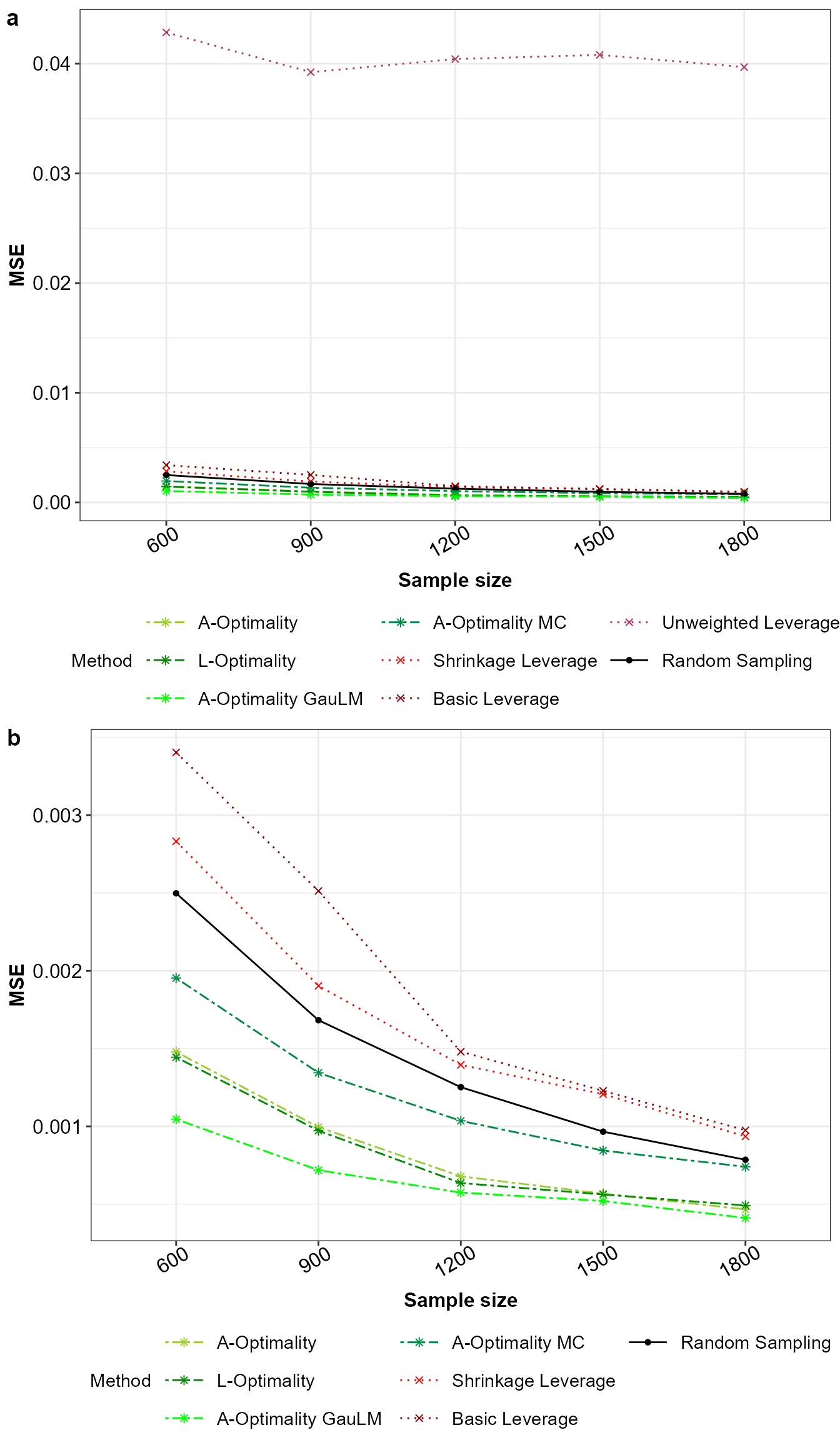
Mean squared error for a) all the sampling methods and b) without unweighted leverage sampling.