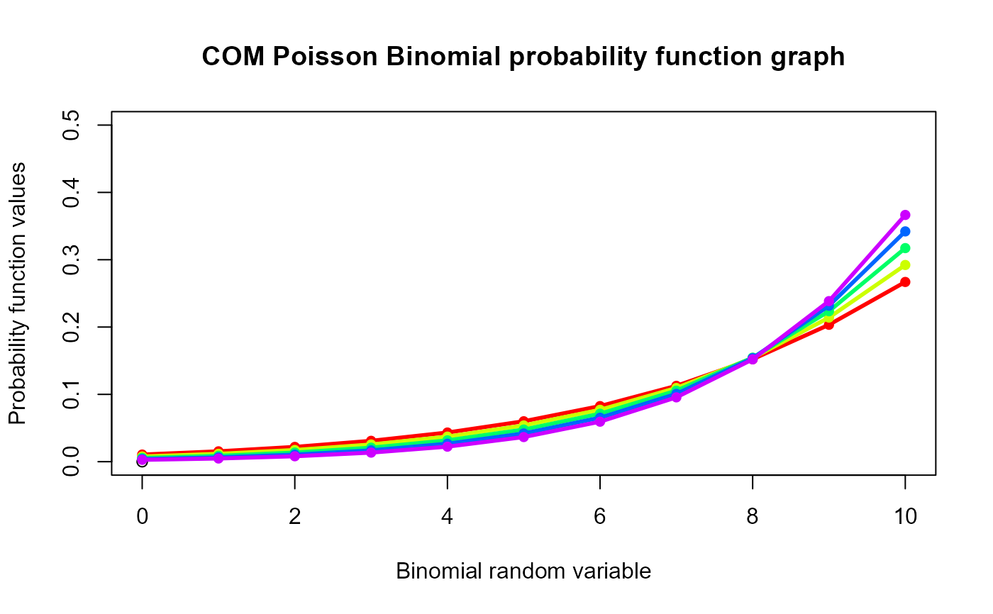
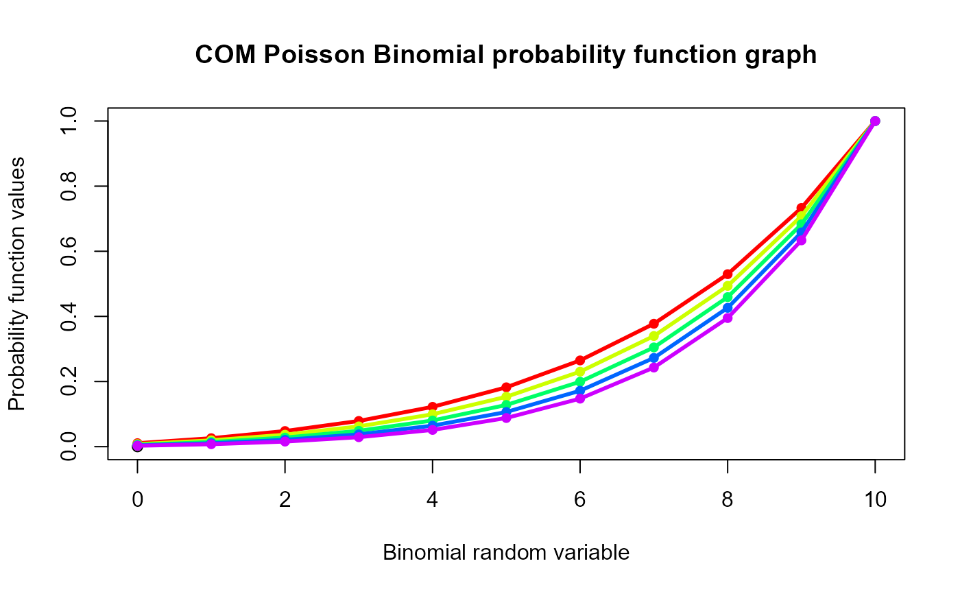
These functions provide the ability for generating probability function values and cumulative probability function values for the COM Poisson Binomial Distribution.
Arguments
- x
vector of binomial random variables.
- n
single value for no of binomial trials.
- p
single value for probability of success.
- v
single value for v.
Details
The probability function and cumulative function can be constructed and are denoted below
The cumulative probability function is the summation of probability function values.
$$P_{COMPBin}(x) = \frac{{n \choose x}^v p^x (1-p)^{n-x}}{\sum_{j=0}^{n} {n \choose j}^v p^j (1-p)^{(n-j)}}$$ $$x = 0,1,2,3,...n$$ $$n = 1,2,3,...$$ $$0 < p < 1$$ $$-\infty < v < +\infty $$
NOTE : If input parameters are not in given domain conditions necessary error messages will be provided to go further.
References
Borges P, Rodrigues J, Balakrishnan N, Bazan J (2014). “A COM--Poisson type generalization of the binomial distribution and its properties and applications.” Statistics and Probability Letters, 87, 158--166.
Examples
#plotting the random variables and probability values
col <- rainbow(5)
a <- c(0.58,0.59,0.6,0.61,0.62)
b <- c(0.022,0.023,0.024,0.025,0.026)
plot(0,0,main="COM Poisson Binomial probability function graph",xlab="Binomial random variable",
ylab="Probability function values",xlim = c(0,10),ylim = c(0,0.5))
for (i in 1:5)
{
lines(0:10,dCOMPBin(0:10,10,a[i],b[i])$pdf,col = col[i],lwd=2.85)
points(0:10,dCOMPBin(0:10,10,a[i],b[i])$pdf,col = col[i],pch=16)
}


dCOMPBin(0:10,10,0.58,0.022)$pdf      #extracting the pdf values
#>  [1] 0.01058483 0.01537669 0.02194887 0.03097149 0.04329998 0.06003554
#>  [7] 0.08257434 0.11263594 0.15222443 0.20337258 0.26697531
dCOMPBin(0:10,10,0.58,0.022)$mean     #extracting the mean
#> [1] 7.627366
dCOMPBin(0:10,10,0.58,0.022)$var      #extracting the variance
#> [1] 5.803804

#plotting the random variables and cumulative probability values
col <- rainbow(5)
a <- c(0.58,0.59,0.6,0.61,0.62)
b <- c(0.022,0.023,0.024,0.025,0.026)
plot(0,0,main="COM Poisson Binomial probability function graph",xlab="Binomial random variable",
ylab="Probability function values",xlim = c(0,10),ylim = c(0,1))
for (i in 1:5)
{
lines(0:10,pCOMPBin(0:10,10,a[i],b[i]),col = col[i],lwd=2.85)
points(0:10,pCOMPBin(0:10,10,a[i],b[i]),col = col[i],pch=16)
}


pCOMPBin(0:10,10,0.58,0.022)      #acquiring the cumulative probability values
#>  [1] 0.01058483 0.02596152 0.04791039 0.07888188 0.12218187 0.18221740
#>  [7] 0.26479174 0.37742768 0.52965211 0.73302469 1.00000000
