Cpdf values of Unit Bounded Distributions or Mixing Distributions
Source:vignettes/Mixing_Distributions_pxxx.Rmd
Mixing_Distributions_pxxx.RmdIT WOULD BE CLEARLY BENEFICIAL FOR YOU BY USING THE RMD FILES IN THE GITHUB DIRECTORY FOR FURTHER EXPLANATION OR UNDERSTANDING OF THE R CODE FOR THE RESULTS OBTAINED IN THE VIGNETTES.
There are few examples for each distribution showing how their Cumulative probability density values change when parameters in concern change. Further they have been plotted so that it would be easy to understand how vivid these Cumulative probability density values change with a slight difference in parameters. The functions which provide the Cpdf values are
-
pUNI- producing Cpdf values for Uniform Distribution. -
pTRI- producing Cpdf values for Triangular Distribution. -
pBETA- producing Cpdf values for Beta Distribution. -
pKUM- producing Cpdf values for Kumaraswamy Distribution. -
pGHGBeta- producing Cpdf values for Gaussian Hyper-geometric Generalized Beta Distribution. -
pGBeta1- producing Cpdf values for Generalized Beta Type 1 Distribution. -
pGAMMA- producing Cpdf values for Gamma Distribution.
Few functions were created for the purpose of plotting Cpdf values. When there are two or more than two shape parameters are involved these functions are used. They are namely.
-
pBETAplot- Function to plot Cpdf values for Beta Distribution. -
pKUMplot- Function to plot Cpdf values for Kumaraswamy Distribution. -
pGHGBetaplot- Function to plot Cpdf values for Gaussian Hyper-geometric Generalized Beta Distribution. -
pGBeta1plot- Function to plot Cpdf values for Generalized Beta Type 1 Distribution. -
pGAMMAplot- Function to plot Cpdf values for Gamma Distribution.
3D plotting will only provide chance to plot limited Cpdf values of few distributions only and it will limit our ability to compare distributions. Therefore new methods should be developed to plot Cpdf values which are generated by two or more shape parameters.
Cumulative Probability Density values for Uniform Distribution
Unit Bounded Uniform distribution does not have any shape parameter. Therefore no significant change in Cpdf values. Although it has been plotted below
prob <- seq(0,1,by=0.05)
pdfv <- pUNI(prob)
data <- data.frame(prob,pdfv)
ggplot(data)+
  geom_line(aes(x=prob,y=pdfv))+
  xlab("Vector of Probabilities")+
  ylab("Cumulative Probability density values")+
  ggtitle("Cpdf values changing")+
  theme_light()+
  scale_x_continuous(breaks=seq(0,1,by=0.1))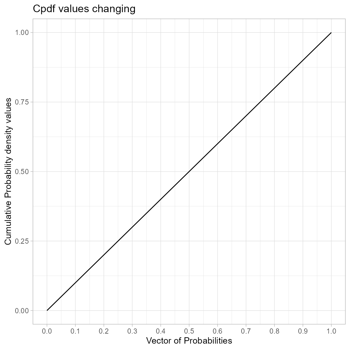
Cumulative Probability Density values for Triangular Distribution
Unit Bounded Triangular distribution has one parameter, which is the mode value in-between zero and one. According to the below given mode parameter value restrictions it has been plotted.
prob <- seq(0.01,0.99,by=0.01)
mode <- seq(0.01,0.99,by=0.01)
output <- matrix(ncol =length(mode) ,nrow=length(prob))
for (i in 1:length(mode))
  {
   output[,i]<-pTRI(prob,mode[i])
  }
data <- data.frame(prob,output)
data <- melt(data,id.vars ="prob" )
ggplot(data,aes(prob,value,col=variable))+
  geom_line()+guides(color="none")+
  xlab("Vector of Probabilities")+
  ylab("Cumulative Probability density values")+
  theme_light()+scale_color_viridis_d()+
  ggtitle("Cpdf values changing when c=seq(0.01,0.09,by0.01)")+
  scale_x_continuous(breaks=seq(0,1,by=0.1))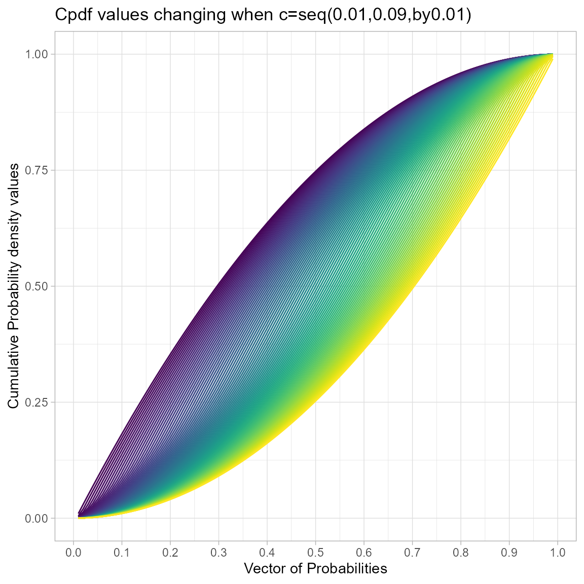
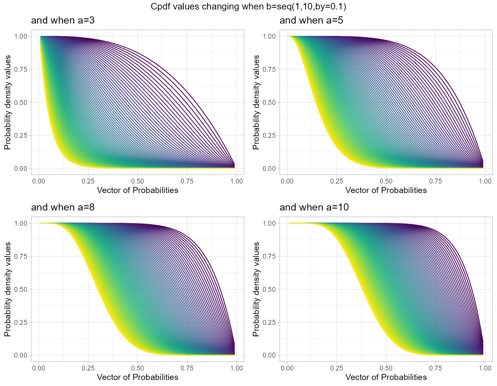
Cumulative Probability Density values for Beta Distribution
Unit Bounded Beta distribution has two shape parameters. These parameters have the ability to provide a very unique set of Cpdf values for each combination of a,b values. Below is a small sample of that reach plotted.
- a,b are in the domain region of above zero.
 b3 <- pBETAplot(a=seq(1,100,by=1),b=3,plot_title="and when b=3",a_seq= T)
 b5 <- pBETAplot(a=seq(1,100,by=1),b=5,plot_title="and when b=5",a_seq= T)
 b8 <- pBETAplot(a=seq(1,100,by=1),b=8,plot_title="and when b=8",a_seq= T)
b10 <- pBETAplot(a=seq(1,100,by=1),b=10,plot_title="and when b=10",a_seq= T)

grid.arrange(b3,b5,b8,b10,nrow=2,top="Cpdf values changing when a=seq(1,100,by=1)")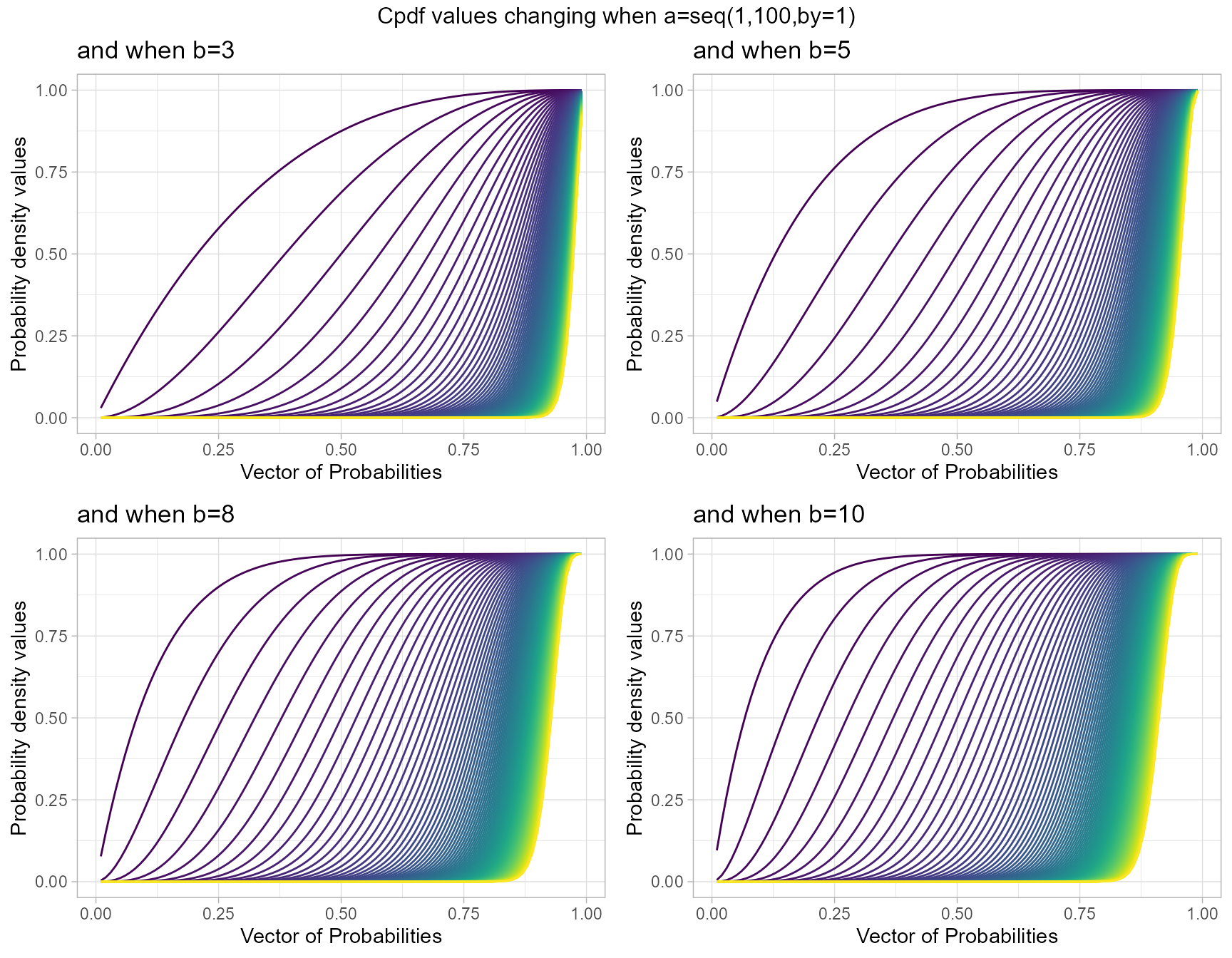
 a3 <- pBETAplot(b=seq(1,100,by=1),a=3,plot_title="and when a=3",a_seq= F)
 a5 <- pBETAplot(b=seq(1,100,by=1),a=5,plot_title="and when a=5",a_seq= F)
 a8 <- pBETAplot(b=seq(1,100,by=1),a=8,plot_title="and when a=8",a_seq= F)
a10 <- pBETAplot(b=seq(1,100,by=1),a=10,plot_title="and when a=10",a_seq= F)

grid.arrange(a3,a5,a8,a10,nrow=2,top="Cpdf values changing when b=seq(1,100,by=1)")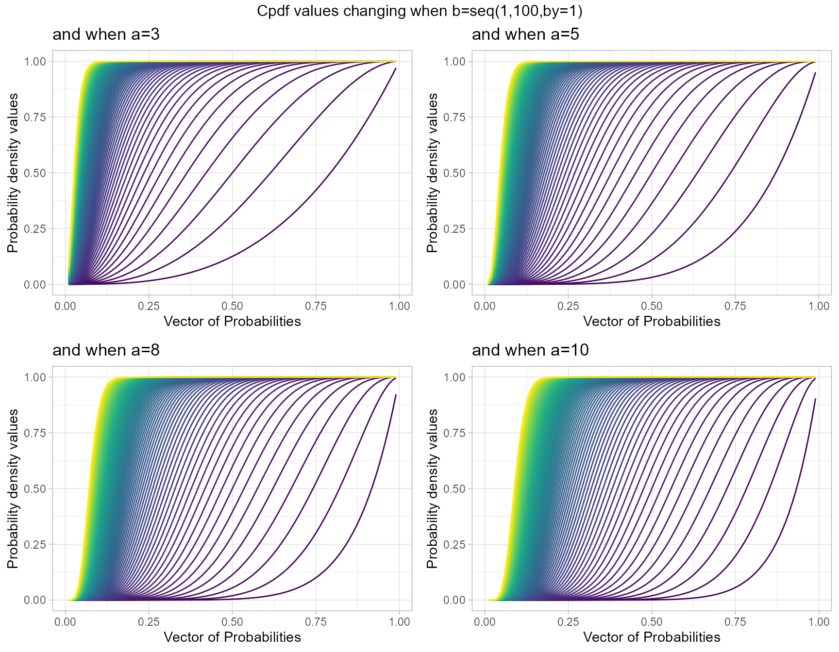
Cumulative Probability Density values for Kumaraswamy Distribution
Similar to Beta distribution the Kumaraswamy distribution also has two shape parameters. It is presumed that Kumaraswamy distribution has the ability to cover more unique Cpdf values than the Beta distribution. Below is a small sample of how Cpdf values change when shape parameters change.
- a,b are in the domain region of above zero.
 b1 <- pKUMplot(a=seq(1,100,by=1),b=1,plot_title="and when b=1",a_seq=T)
 b2 <- pKUMplot(a=seq(1,100,by=1),b=2,plot_title="and when b=2",a_seq=T)
 b5 <- pKUMplot(a=seq(1,100,by=1),b=5,plot_title="and when b=5",a_seq=T)
b10 <- pKUMplot(a=seq(1,100,by=1),b=10,plot_title="and when b=10",a_seq=T)

grid.arrange(b1,b2,b5,b10,nrow=2,top="Cpdf values changing when a=seq(1,100,by=1)")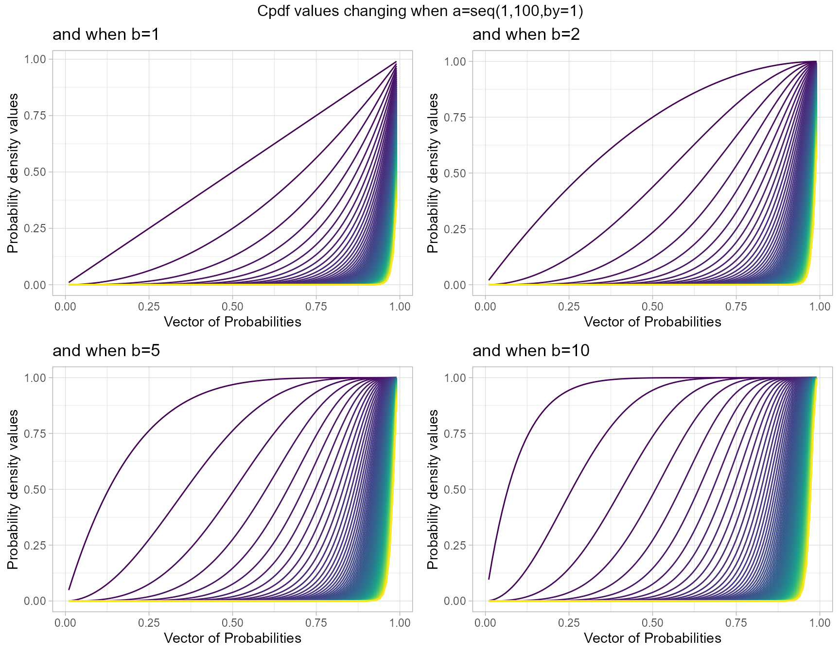
 a3 <- pKUMplot(b=seq(1,100,by=1),a=3,plot_title="and when a=3",a_seq=F)
 a5 <- pKUMplot(b=seq(1,100,by=1),a=5,plot_title="and when a=5",a_seq=F)
a10 <- pKUMplot(b=seq(1,100,by=1),a=10,plot_title="and when a=10",a_seq=F)
a15 <- pKUMplot(b=seq(1,100,by=1),a=13,plot_title="and when a=15",a_seq=F)

grid.arrange(a3,a10,a10,a15,nrow=2,top="Cpdf values changing when b=seq(1,100,by=1)")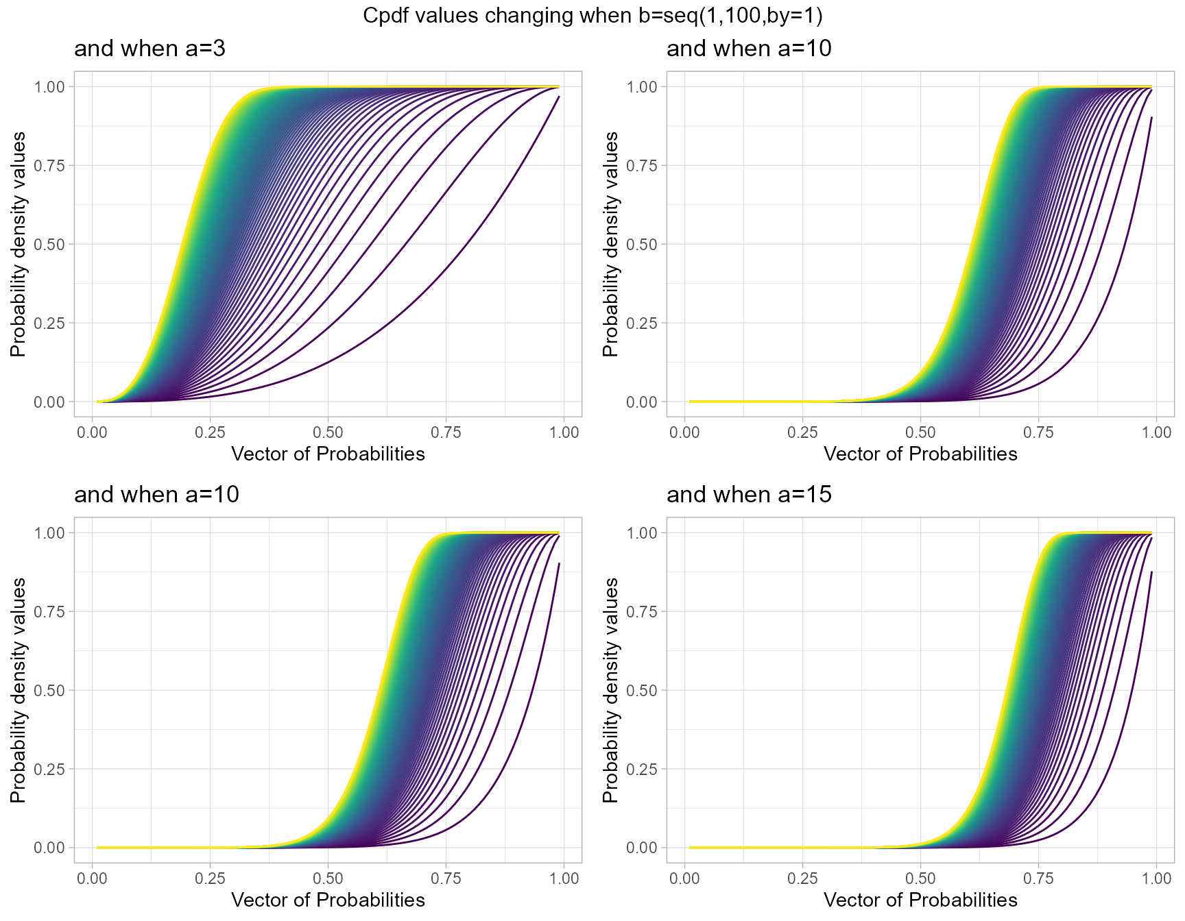
Cumulative Probability Density values for Gaussian Hyper-geometric Generalized Beta Distribution
Unlike the previous mentioned distributions Gaussian Hyper-geometric Generalized Beta Distribution was not developed first hand. It is a by product of Gaussian Hyper-geometric Generalized Beta Binomial (GHGBB) Distribution. There are three shape parameters, which are a,b,c and a binomial trial value called n. Below is a brief account of how the Cpdf values evolve with shape parameters change.
- a,b,c are in the domain region of above zero.
- n is a natural number which should only take values of 0,1,2,… .
 b10c5 <- pGHGBetaplot(n=10,a=seq(.1,100,by=.1),b=10,c=5,
                    plot_title="and when b=10, c=5",a_seq=T,b_seq=F)
 b50c5 <- pGHGBetaplot(n=10,a=seq(.1,100,by=.1),b=50,c=5,
                    plot_title="and when b=50, c=5",a_seq=T,b_seq=F)
b100c5 <- pGHGBetaplot(n=10,a=seq(.1,100,by=.1),b=100,c=5,
                     plot_title="and when b=100, c=5",a_seq=T,b_seq=F)
b150c5 <- pGHGBetaplot(n=10,a=seq(.1,100,by=.1),b=150,c=5,
                     plot_title="and when b=150, c=5",a_seq=T,b_seq=F)

grid.arrange(b10c5,b50c5,b100c5,b150c5,nrow=2,
             top="Cpdf values changing when a=seq(0.1,100,by=0.1)")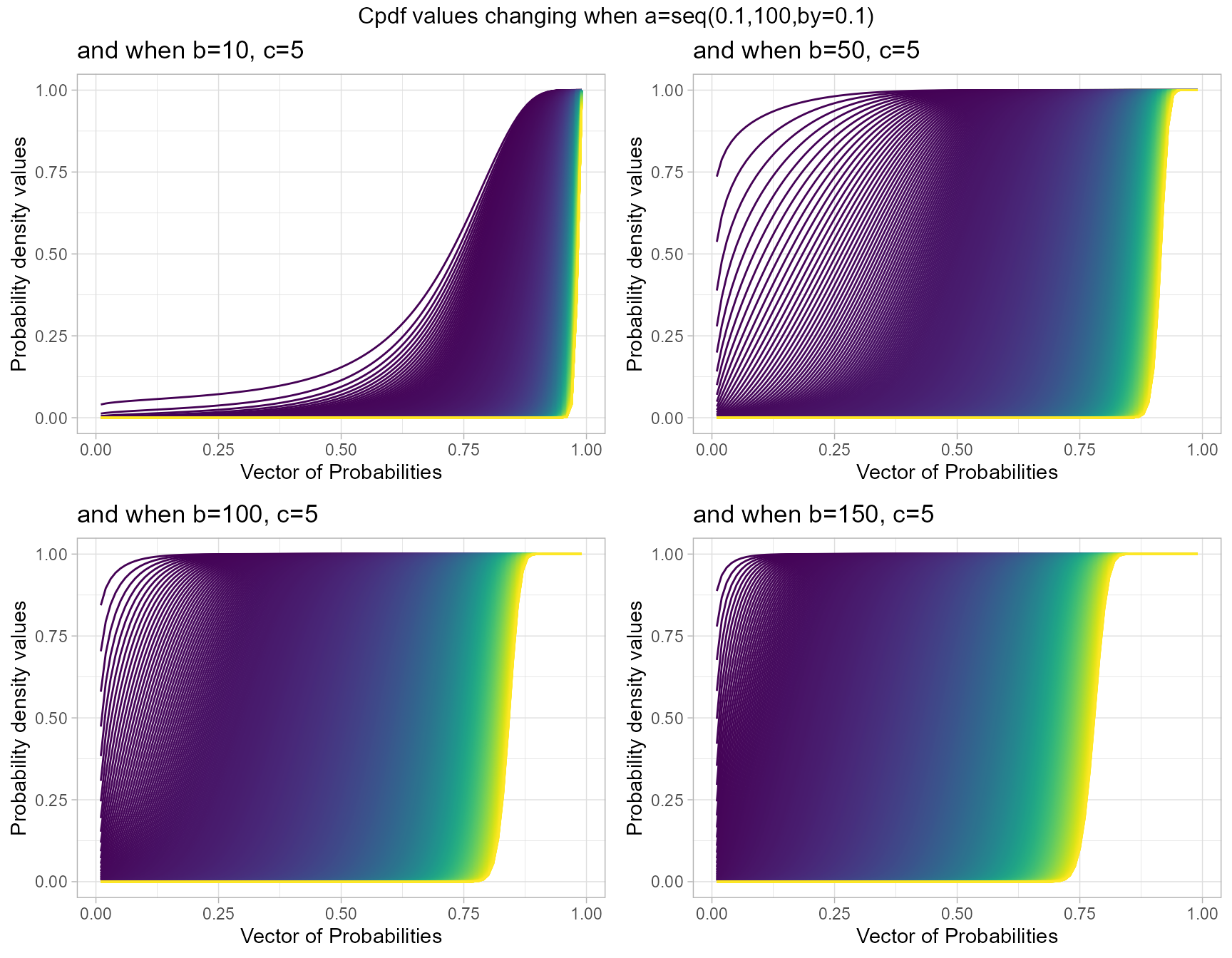
 b40c10 <- pGHGBetaplot(n=10,a=seq(.1,100,by=.1),b=40,c=10,
                     plot_title="and when b=40, c=10",a_seq=T,b_seq=F)
 b50c10 <- pGHGBetaplot(n=10,a=seq(.1,100,by=.1),b=50,c=10,
                     plot_title="and when b=50, c=10",a_seq=T,b_seq=F)
b100c10 <- pGHGBetaplot(n=10,a=seq(.1,100,by=.1),b=100,c=10,
                      plot_title="and when b=100, c=10",a_seq=T,b_seq=F)
b200c10 <- pGHGBetaplot(n=10,a=seq(.1,100,by=.1),b=200,c=10,
                      plot_title="and when b=200, c=10",a_seq=T,b_seq=F)

grid.arrange(b40c10,b50c10,b100c10,b200c10,nrow=2,
             top="Cpdf values changing when a=seq(0.1,100,by=0.1)")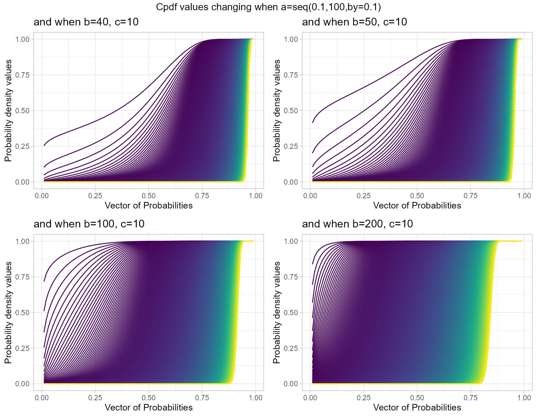
Cumulative Probability Density values for Generalized Beta Type1 Distribution
Generalized Beta Type 1 distribution is a latest achievement of unit bounded distributions. It has three shape parameters which are a, b and c. Below is a very small variation of Cpdf values for the mentioned a,b and c shape parameters values plotted.
- a,b,c in the domain region of above zero.
 b1c0.3 <- pGBeta1plot(a=seq(1,40,by=0.1),b=1,c=0.3,
                      plot_title="and when b=1, c=0.3",a_seq=T,b_seq=F)
 b1c0.4 <- pGBeta1plot(a=seq(1,40,by=0.1),b=1,c=0.4,
                      plot_title="and when b=1, c=0.4",a_seq=T,b_seq=F)
 b1c0.5 <- pGBeta1plot(a=seq(1,40,by=0.1),b=1,c=0.5,
                      plot_title="and when b=1, c=0.5",a_seq=T,b_seq=F)
b1c0.55 <- pGBeta1plot(a=seq(1,40,by=0.1),b=1,c=0.55,
                      plot_title="and when b=1, c=0.55",a_seq=T,b_seq=F)

grid.arrange(b1c0.3,b1c0.4,b1c0.5,b1c0.55,nrow=2,
             top="Cpdf values changing when a=seq(1,40,by=0.1)")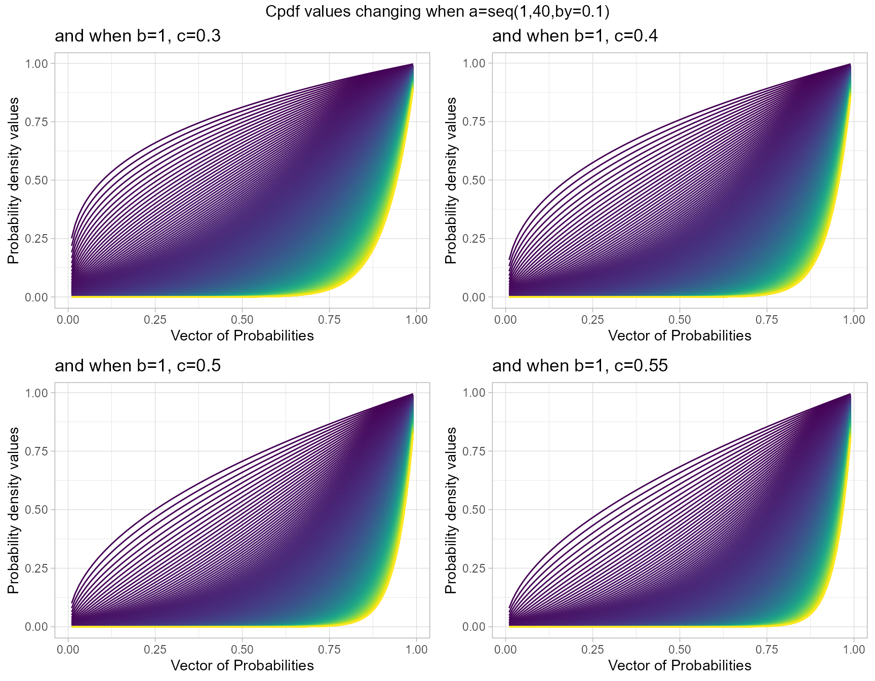
  b1c1 <- pGBeta1plot(a=seq(.5,100,by=.1),b=1,c=1,
                    plot_title="and when b=1, c=1",a_seq=T,b_seq=F)
b1c1.5 <- pGBeta1plot(a=seq(.5,100,by=.1),b=1,c=1.5,
                    plot_title="and when b=1, c=1.5",a_seq=T,b_seq=F)
  b1c2 <- pGBeta1plot(a=seq(.5,100,by=.1),b=1,c=2,
                    plot_title="and when b=1, c=2",a_seq=T,b_seq=F)
b1c2.5 <- pGBeta1plot(a=seq(.5,100,by=.1),b=1,c=2.5,
                    plot_title="and when b=1, c=2.5",a_seq=T,b_seq=F)

grid.arrange(b1c1,b1c1.5,b1c2,b1c2.5,nrow=2,
             top="Cpdf values changing when a=seq(0.5,100,by=0.1)")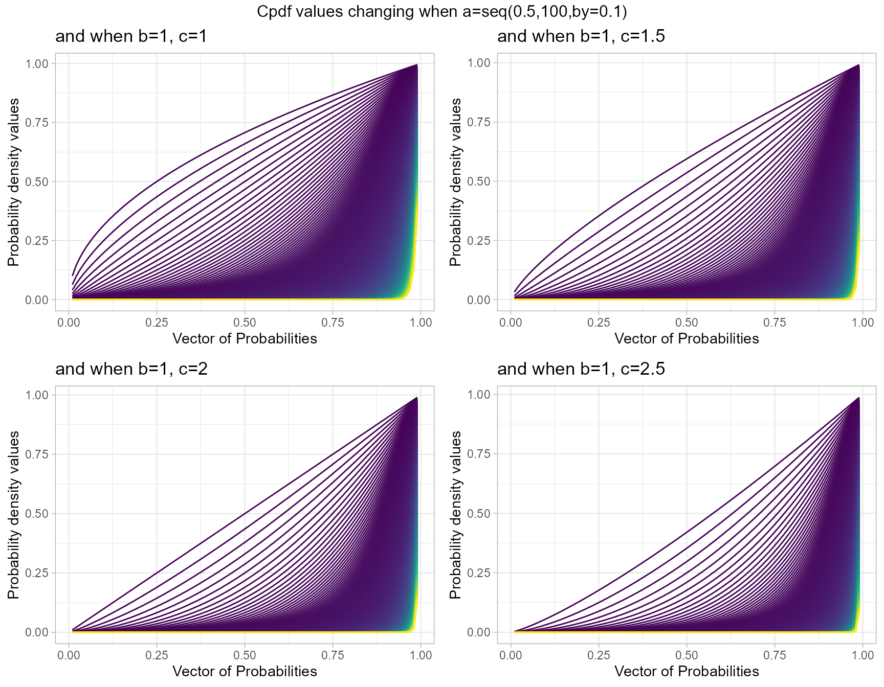
Cumulative Probability Density values for Gamma Distribution
Unit Bounded Gamma distribution has two shape parameters. These parameters have the ability to provide a very unique set of Cpdf values for each combination of a,b values. Below is a small sample of that reach plotted.
- a,b are in the domain region of above zero.
 b3 <- pGAMMAplot(a=seq(1,10,by=0.5),b=3,plot_title="and when b=3",a_seq= T)
 b5 <- pGAMMAplot(a=seq(1,10,by=0.5),b=5,plot_title="and when b=5",a_seq= T)
 b8 <- pGAMMAplot(a=seq(1,10,by=0.5),b=8,plot_title="and when b=8",a_seq= T)
b10 <- pGAMMAplot(a=seq(1,10,by=0.5),b=10,plot_title="and when b=10",a_seq= T)

grid.arrange(b3,b5,b8,b10,nrow=2,top="Cpdf values changing when a=seq(1,10,by=0.5)")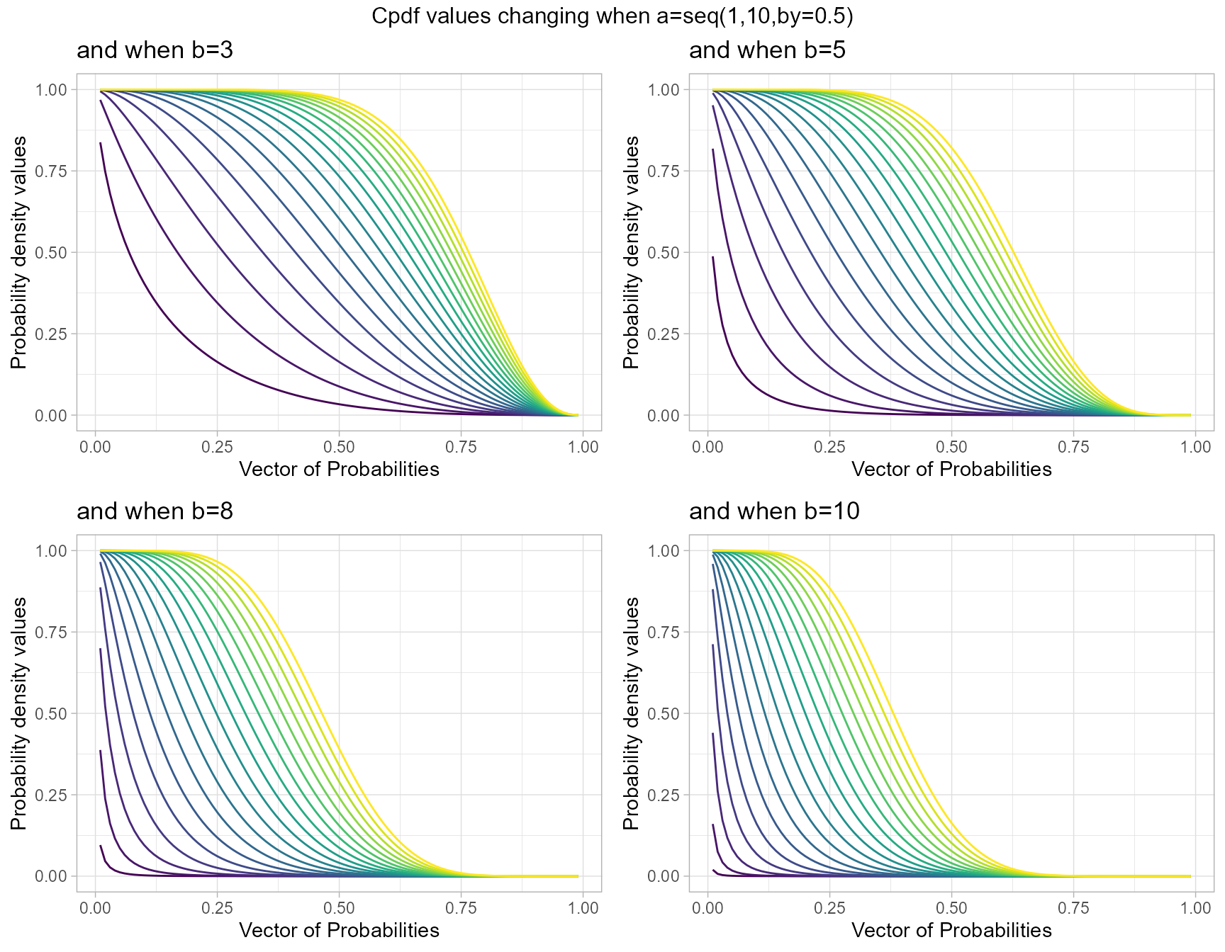
 a3 <- pGAMMAplot(b=seq(1,10,by=0.1),a=3,plot_title="and when a=3",a_seq= F)
 a5 <- pGAMMAplot(b=seq(1,10,by=0.1),a=5,plot_title="and when a=5",a_seq= F)
 a8 <- pGAMMAplot(b=seq(1,10,by=0.1),a=8,plot_title="and when a=8",a_seq= F)
a10 <- pGAMMAplot(b=seq(1,10,by=0.1),a=10,plot_title="and when a=10",a_seq= F)

grid.arrange(a3,a5,a8,a10,nrow=2,top="Cpdf values changing when b=seq(1,10,by=0.1)")