Binomial Mixture and Alternate Binomial Distributions CPMF values
Source:vignettes/BMDs_and_ABDs_pxxxBin.Rmd
BMDs_and_ABDs_pxxxBin.RmdIT WOULD BE CLEARLY BENEFICIAL FOR YOU BY USING THE RMD FILES IN THE GITHUB DIRECTORY FOR FURTHER EXPLANATION OR UNDERSTANDING OF THE R CODE FOR THE RESULTS OBTAINED IN THE VIGNETTES.
# Binomial Mixture Distributions
Cumulative probability mass function values are calculated using probability mass function values. Here also in order to understand the variation of distributions plots have been used. The functions which can develop the Cpmf values are
-
pUniBin- producing Cpmf values for Uniform Binomial Distribution. -
pTriBin- producing Cpmf values for Triangular Binomial Distribution. -
pBetaBin- producing Cpmf values for Beta-Binomial Distribution. -
pKumBin- producing Cpmf values for Kumaraswamy Binomial Distribution. -
pGHGBB- producing Cpmf values for Gaussian Hyper-geometric Generalized Beta-Binomial Distribution. -
pMcGBB- producing Cpmf values for McDonald Generalized Beta-Binomial Distribution. -
pGammaBin- producing Cpmf values for Gamma Binomial Distribution. -
pGrassiaIIBin- producing Cpmf values for Grassia II Binomial Distribution.
Special functions have been developed to generate plots with related to distributions with more than one parameter. These functions are
-
pBetaBinplot- plot function to Beta-Binomial Distribution. -
pKumBinplot- plot function to Kumaraswamy Binomial Distribution. -
pGHGBBplot- plot function to Gaussian Hyper-geometric Generalized Beta-Binomial Distribution. -
pMcGBBplot- plot function to McDonald Generalized Beta-Binomial Distribution. -
pGammaBinplot- plot function to Gamma Binomial Distribution. -
pGrassiaIIBinplot- plot function to Grassia II Binomial Distribution.
Cumulative Probability Mass Function values for Uniform Binomial Distribution
Uniform Binomial distribution does not provide very wide variety of Cpmf values such as other distributions. Still the plot of Cpmf values with related to binomial random variable is given below
brv <- 0:10
cpmfv <- pUniBin(brv,max(brv))
data <- data.frame(brv,cpmfv)
ggplot(data,aes(x=brv,y=cpmfv))+
  geom_line()+
  xlab("Binomial Random Variable")+
  ylab("Cumulative Probability Mass Function values")+
  ggtitle("Cpmf values changing")+
  theme_light()+
  scale_x_continuous(breaks=seq(0,10,by=1))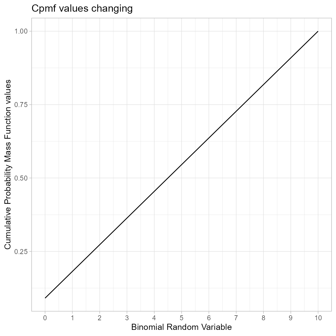
Cumulative Probability Mass Function values for Triangular Binomial Distribution
With one parameter, which is the mode value for Triangular Binomial Distribution in-between zero and one. There is very limited amount of Cpmf values for the change in mode parameter. Plot for Cpmf values with relative to binomial random variable is given below
brv <- seq(0,15,by=1)
mode <- seq(0.02,0.98,by=0.01)
output <- matrix(ncol =length(mode) ,nrow=length(brv))
for (i in 1:length(mode))
  {
   output[,i]<-pTriBin(brv,max(brv),mode[i])
  }
data <- data.frame(brv,output)
data <- melt(data,id.vars ="brv" )
ggplot(data,aes(brv,value,col=variable))+
  geom_line()+guides(fill=FALSE,color=FALSE)+
  xlab("Binomial Random Variable")+
  ylab("Cumulative Probability Mass values")+
  theme_light()+scale_color_viridis_d()+
  ggtitle("Cpmf values changing for c=seq(0.02,0.98,by=0.01)")
## Warning: The `<scale>` argument of `guides()` cannot be `FALSE`. Use "none" instead as
## of ggplot2 3.3.4.
## This warning is displayed once every 8 hours.
## Call `lifecycle::last_lifecycle_warnings()` to see where this warning was
## generated.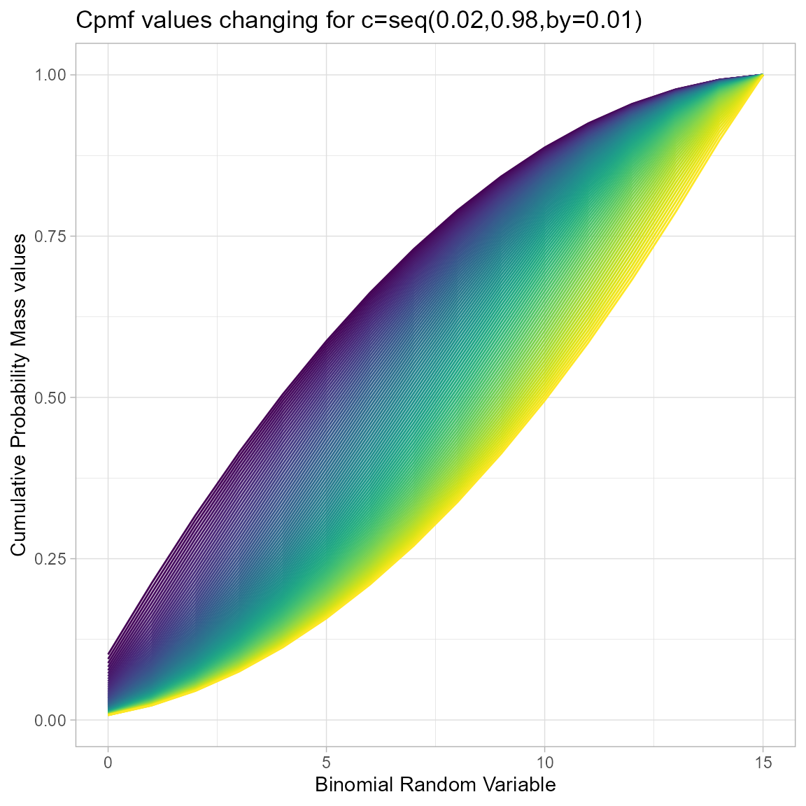
scale_x_continuous(breaks=seq(0,15,by=1))## <ScaleContinuousPosition>
## Range:
## Limits: 0 -- 1Cumulative Probability Mass Function values for Beta-Binomial Distribution
Beta-Binomial with two shape parameters a and b have more vivid Cpmf value patterns than Triangular Binomial distribution. It can be clearly seen in the given plot below.
- a,b are in the domain region of above zero.
 b10 <- pBetaBinplot(a=seq(1,100,by=1),b=10,plot_title="and when b=10",a_seq= T)
 b50 <- pBetaBinplot(a=seq(1,100,by=1),b=50,plot_title="and when b=50",a_seq= T)
b100 <- pBetaBinplot(a=seq(1,100,by=1),b=100,plot_title="and when b=100",a_seq= T)
b200 <- pBetaBinplot(a=seq(1,100,by=1),b=200,plot_title="and when b=200",a_seq= T)

grid.arrange(b10,b50,b100,b200,nrow=2,top="Cpmf values changing when a=seq(1,100,by=1)")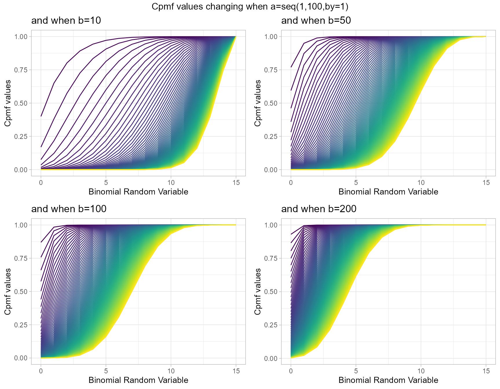
 a10 <- pBetaBinplot(b=seq(1,100,by=1),a=10,plot_title="and when a=10",a_seq= F)
 a50 <- pBetaBinplot(b=seq(1,100,by=1),a=50,plot_title="and when a=50",a_seq= F)
a100 <- pBetaBinplot(b=seq(1,100,by=1),a=100,plot_title="and when a=100",a_seq= F)
a200 <- pBetaBinplot(b=seq(1,100,by=1),a=200,plot_title="and when a=200",a_seq= F)

grid.arrange(a10,a50,a100,a200,nrow=2,top="Cpmf values changing when b=seq(1,100,by=1)")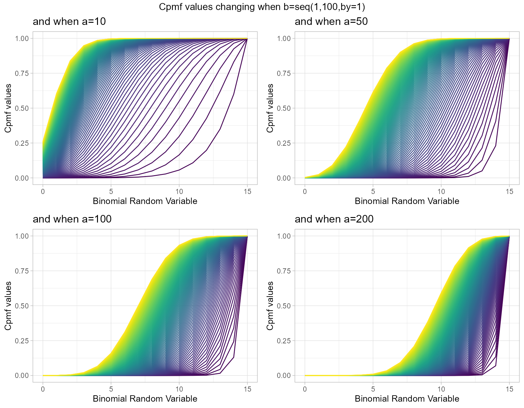
Cumulative Probability Mass Function values for Kumaraswamy Binomial Distribution
Similarly parameters such as Beta-Binomial distribution yet holding more Cpmf values is a clear advantage mentioned towards Kumaraswamy Binomial distribution. It also has the parameters a and b. Below is a small demonstration using plots to show how Cpmf values change
- a,b are in the domain region of above zero.
 b5 <- pKumBinplot(a=seq(1,50,by=1),b=5,plot_title="and when b=5",a_seq=T)
b10 <- pKumBinplot(a=seq(1,50,by=1),b=10,plot_title="and when b=10",a_seq=T)
b20 <- pKumBinplot(a=seq(1,50,by=1),b=20,plot_title="and when b=20",a_seq=T)
b25 <- pKumBinplot(a=seq(1,50,by=1),b=25,plot_title="and when b=25",a_seq=T)

grid.arrange(b5,b10,b10,b25,nrow=2,top="Cpmf values changing when a=seq(1,50,by=1)")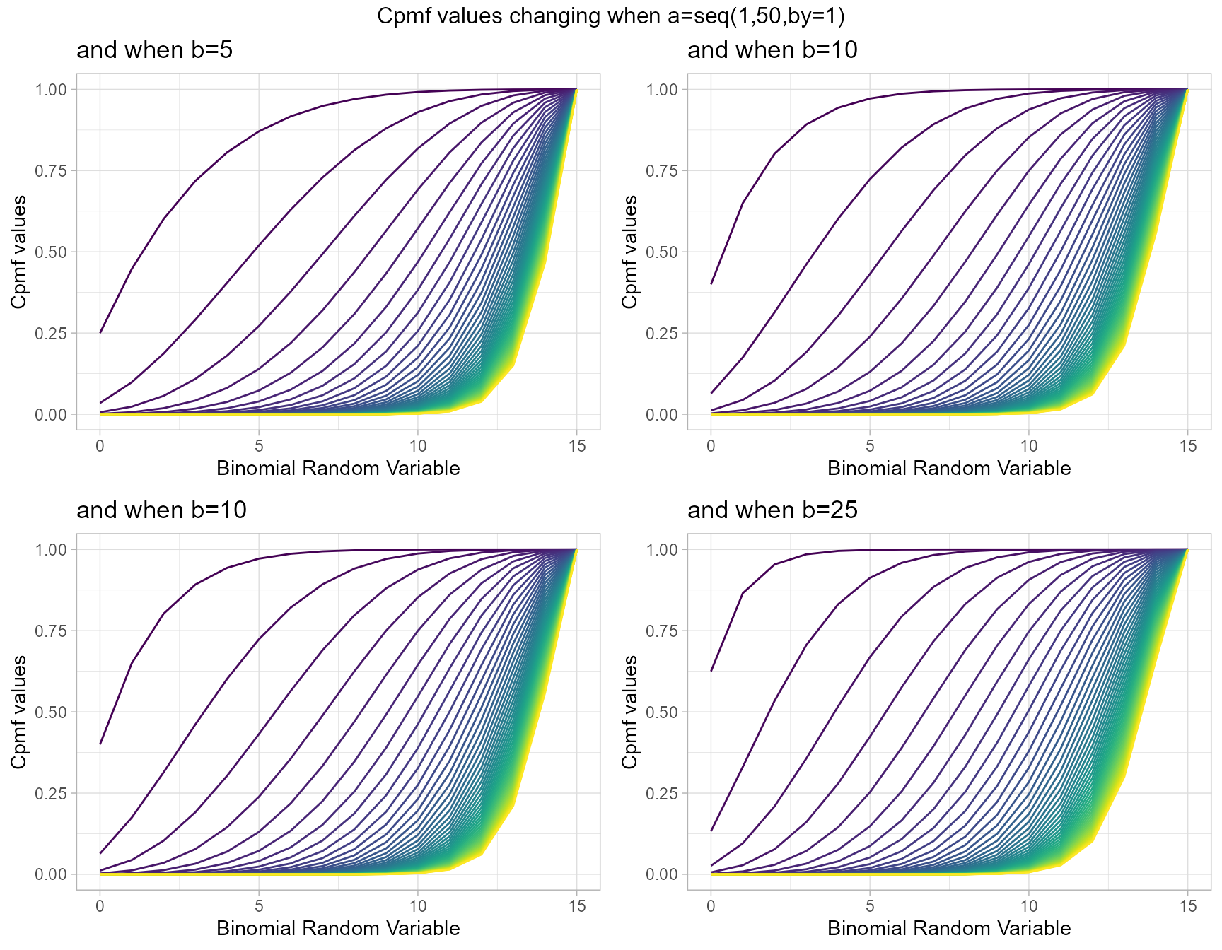
 a5 <- pKumBinplot(b=seq(1,30,by=1),a=5,plot_title="and when a=5",a_seq=F)
a10 <- pKumBinplot(b=seq(1,30,by=1),a=10,plot_title="and when a=10",a_seq=F)
a20 <- pKumBinplot(b=seq(1,30,by=1),a=20,plot_title="and when a=20",a_seq=F)
a25 <- pKumBinplot(b=seq(1,30,by=1),a=25,plot_title="and when a=25",a_seq=F)

grid.arrange(a5,a10,a20,a25,nrow=2,top="Cpmf values changing when b=seq(1,30,by=1)")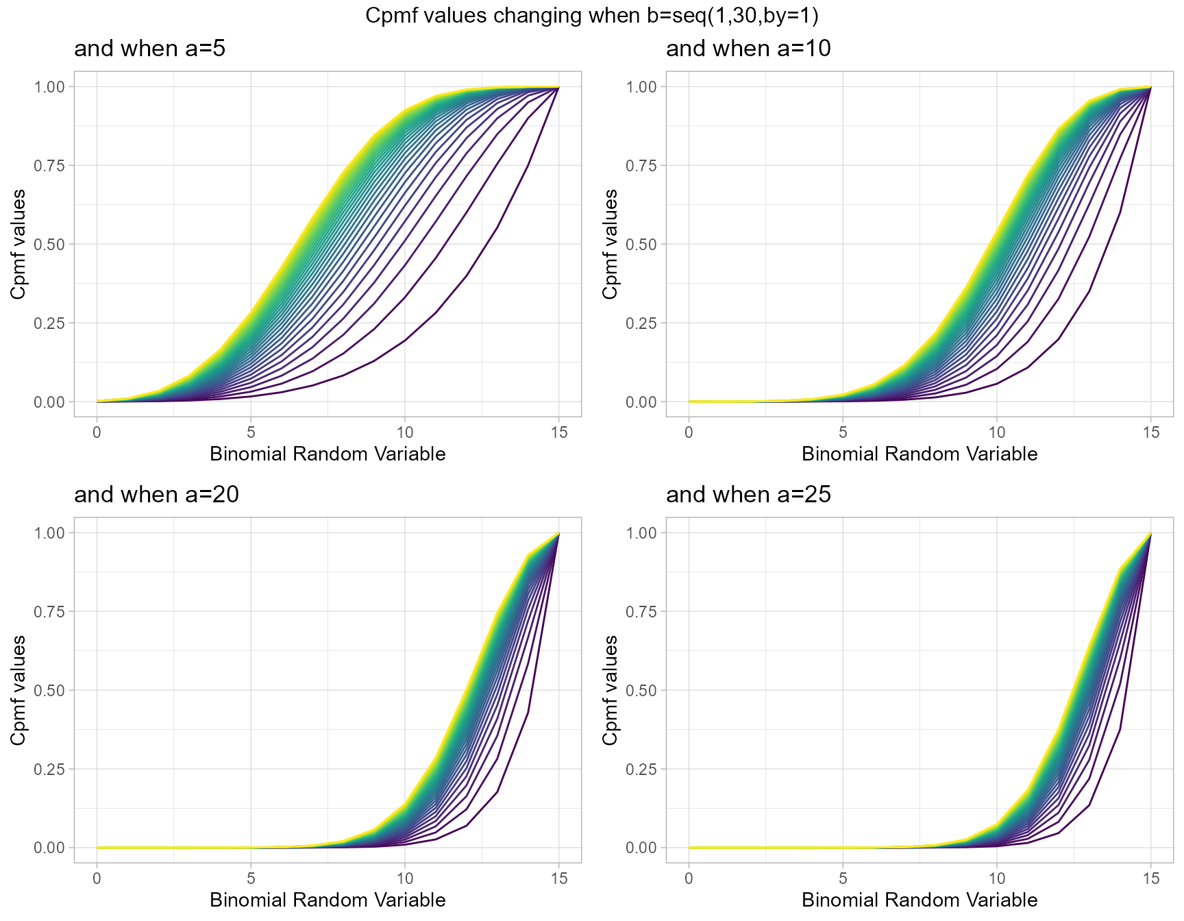
Cumulative Probability Mass Function values for Gaussian Hyper-geometric Generalized Beta-Binomial Distribution
Gaussian Hyper-geometric series function plays a massive role in generating Cpmf values here. There are three parameters in use of this distribution they are a,b and c. Below is a series Cpmf values plotted with respective to shape parameters
- a,b,c are in the domain region of above zero.
 b10c5 <- pGHGBBplot(a=seq(.1,100,by=.1),b=10,c=5,
                  plot_title="and when b=10, c=5",a_seq=T,b_seq=F)
 b50c5 <- pGHGBBplot(a=seq(.1,100,by=.1),b=50,c=5,
                  plot_title="and when b=50, c=5",a_seq=T,b_seq=F)
b100c5 <- pGHGBBplot(a=seq(.1,100,by=.1),b=100,c=5,
                   plot_title="and when b=100, c=5",a_seq=T,b_seq=F)
b150c5 <- pGHGBBplot(a=seq(.1,100,by=.1),b=150,c=5,
                   plot_title="and when b=150, c=5",a_seq=T,b_seq=F)

grid.arrange(b10c5,b50c5,b100c5,b150c5,nrow=2,
             top="Cpmf values changing when a=seq(0.1,100,by=0.1)")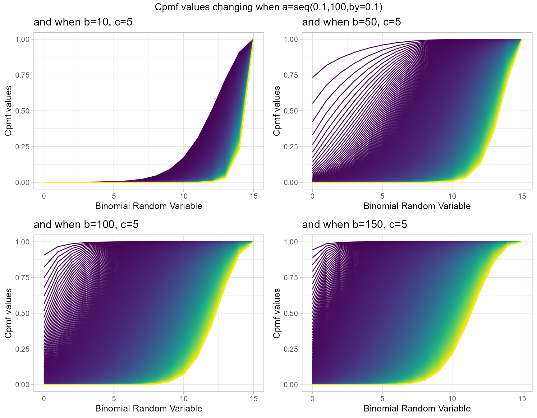
 b10c10 <- pGHGBBplot(a=seq(.1,100,by=.1),b=10,c=10,
                   plot_title="and when b=10, c=10",a_seq=T,b_seq=F)
 b50c10 <- pGHGBBplot(a=seq(.1,100,by=.1),b=50,c=10,
                   plot_title="and when b=50, c=10",a_seq=T,b_seq=F)
b100c10 <- pGHGBBplot(a=seq(.1,100,by=.1),b=100,c=10,
                    plot_title="and when b=100, c=10",a_seq=T,b_seq=F)
b200c10 <- pGHGBBplot(a=seq(.1,100,by=.1),b=200,c=10,
                    plot_title="and when b=200, c=10",a_seq=T,b_seq=F)

grid.arrange(b10c10,b50c10,b100c10,b200c10,nrow=2,
             top="Cpmf values changing when a=seq(0.1,100,by=0.1)")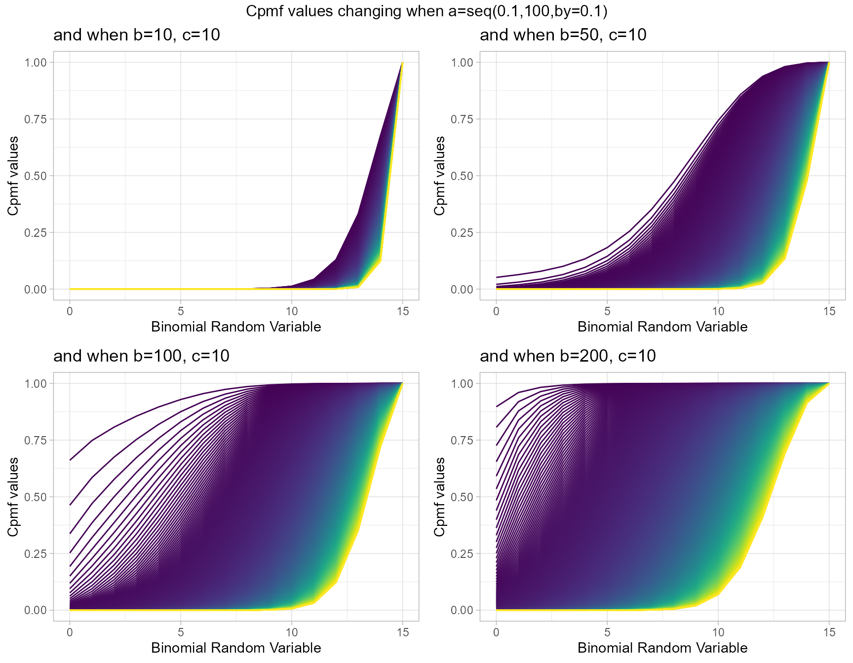
Cumulative Probability Mass Function values for McDonald Generalized Beta-Binomial Distribution
Similar to GHGBB distribution this also has three shape parameters, they are a,b and c. They are very useful in generating vivid Cpmf values. Below given plots describes them most
- a,b,c are in the domain region of above zero.
  b1c5 <- pMcGBBplot(a=seq(.5,10,by=.1),b=1,c=5,
                   plot_title="and when b=1, c=5",a_seq=T,b_seq=F)
b1.2c5 <- pMcGBBplot(a=seq(.5,10,by=.1),b=1.2,c=5,
                   plot_title="and when b=1.2, c=5",a_seq=T,b_seq=F)
  b3c5 <- pMcGBBplot(a=seq(.5,10,by=.1),b=3,c=5,
                   plot_title="and when b=3, c=5",a_seq=T,b_seq=F)
b3.2c5 <- pMcGBBplot(a=seq(.5,10,by=.1),b=3.2,c=5,
                   plot_title="and when b=3.2, c=5",a_seq=T,b_seq=F)

grid.arrange(b1c5,b1.2c5,b3c5,b3.2c5,nrow=2,
             top="Cpmf values changing when a=seq(0.5,10,by=0.1)")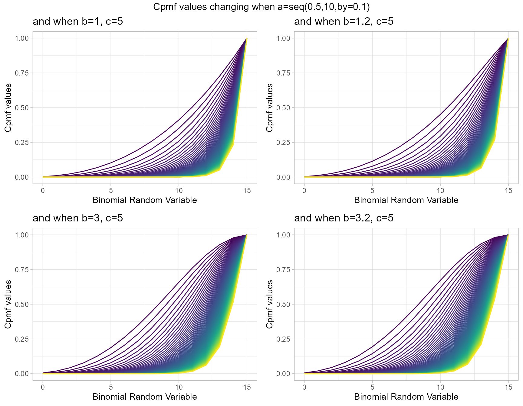
  b1c1 <- pMcGBBplot(a=seq(.5,100,by=.1),b=1,c=1,
                   plot_title="and when b=1, c=1",a_seq=T,b_seq=F)
b1c1.5 <- pMcGBBplot(a=seq(.5,100,by=.1),b=1,c=1.5,
                   plot_title="and when b=1, c=1.5",a_seq=T,b_seq=F)
  b1c2 <- pMcGBBplot(a=seq(.5,100,by=.1),b=1,c=2,
                   plot_title="and when b=1, c=2",a_seq=T,b_seq=F)
b1c2.5 <- pMcGBBplot(a=seq(.5,100,by=.1),b=1,c=2.5,
                   plot_title="and when b=1, c=2.5",a_seq=T,b_seq=F)

grid.arrange(b1c1,b1c1.5,b1c2,b1c2.5,nrow=2,
             top="Cpmf values changing when a=seq(0.5,100,by=0.1)")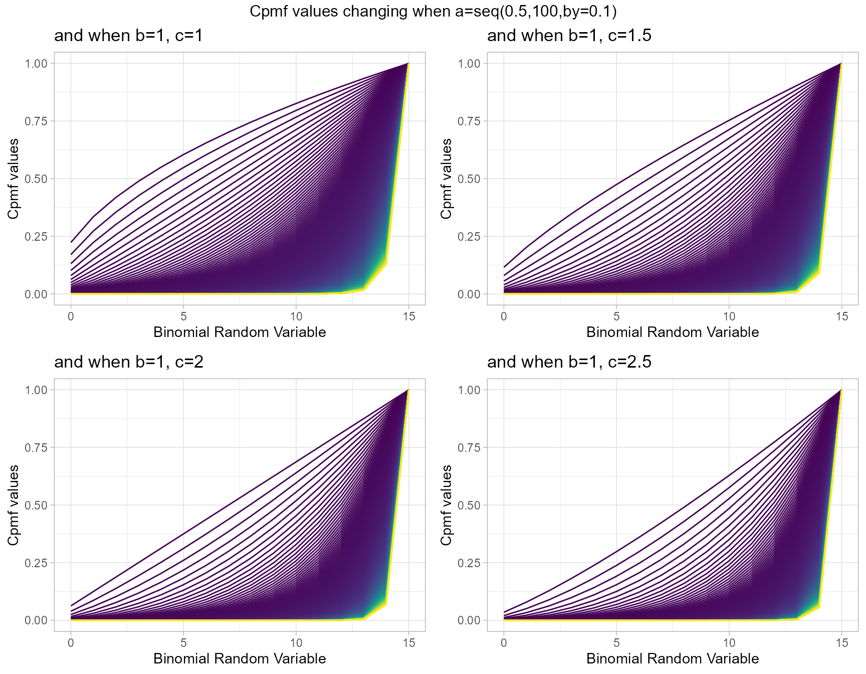
Cumulative Probability Mass Function values for Gamma Binomial Distribution
Gamma Binomial with two shape parameters a and b have more vivid Cpmf value patterns than Triangular Binomial distribution. It can be clearly seen in the given plot below.
- a,b are in the domain region of above zero.
 b10 <- pGammaBinplot(a=seq(1,100,by=1),b=10,plot_title="and when b=10",a_seq= T)
 b50 <- pGammaBinplot(a=seq(1,100,by=1),b=50,plot_title="and when b=50",a_seq= T)
b100 <- pGammaBinplot(a=seq(1,100,by=1),b=100,plot_title="and when b=100",a_seq= T)
b200 <- pGammaBinplot(a=seq(1,100,by=1),b=200,plot_title="and when b=200",a_seq= T)

grid.arrange(b10,b50,b100,b200,nrow=2,top="Cpmf values changing when a=seq(1,100,by=1)")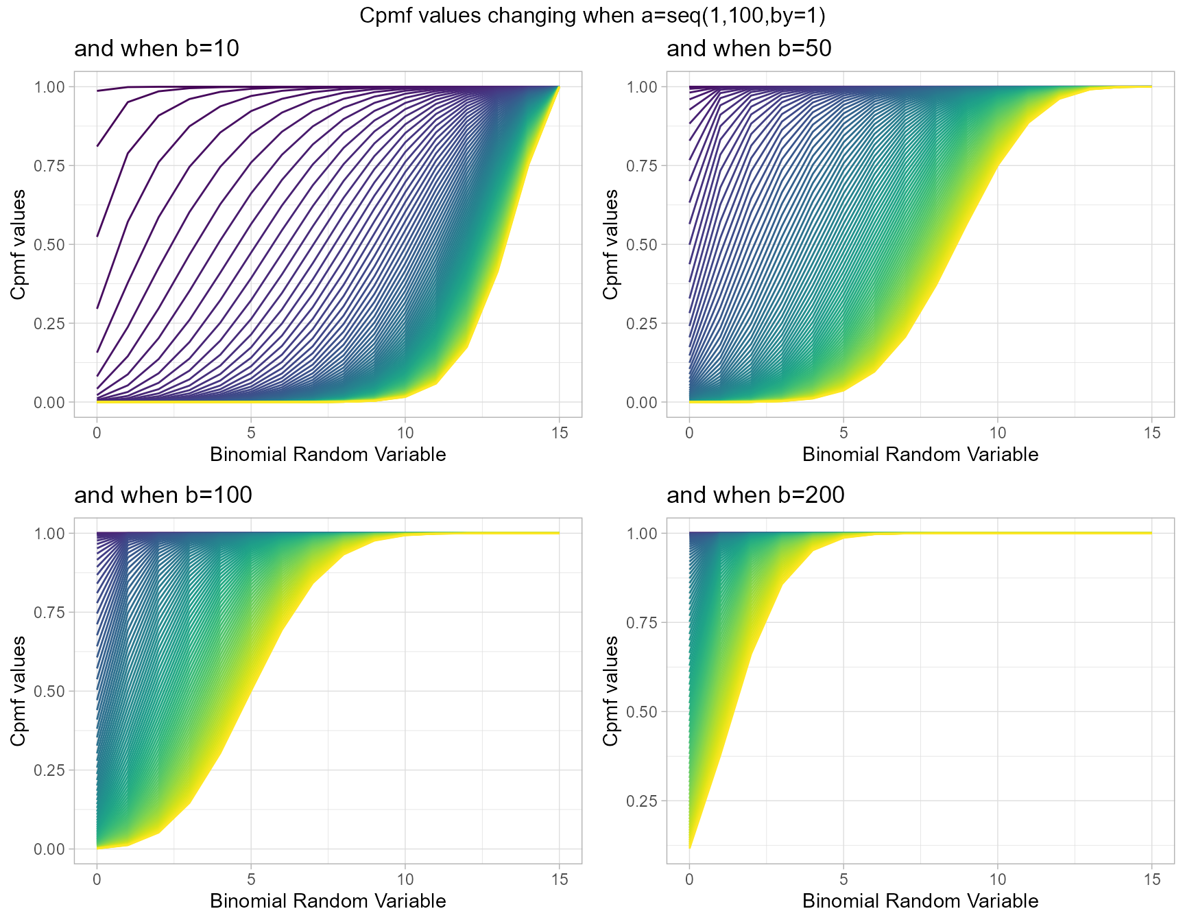
 a10 <- pGammaBinplot(b=seq(1,100,by=1),a=10,plot_title="and when a=10",a_seq= F)
 a50 <- pGammaBinplot(b=seq(1,100,by=1),a=50,plot_title="and when a=50",a_seq= F)
a100 <- pGammaBinplot(b=seq(1,100,by=1),a=100,plot_title="and when a=100",a_seq= F)
a200 <- pGammaBinplot(b=seq(1,100,by=1),a=200,plot_title="and when a=200",a_seq= F)

grid.arrange(a10,a50,a100,a200,nrow=2,top="Cpmf values changing when b=seq(1,100,by=1)")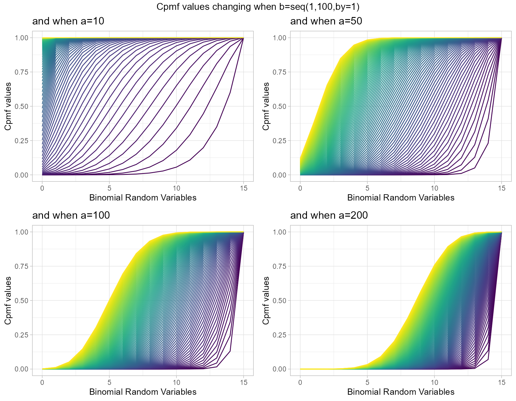
Cumulative Probability Mass Function values for Grassia II Binomial Distribution
Grassia II Binomial with two shape parameters a and b have more vivid Cpmf value patterns than Triangular Binomial distribution. It can be clearly seen in the given plot below.
- a,b are in the domain region of above zero.
 b1 <- pGrassiaIIBinplot(a=seq(0.1,10,by=0.1),b=0.1,plot_title="and when b=0.1",a_seq= T)
b25 <- pGrassiaIIBinplot(a=seq(0.1,10,by=0.1),b=0.25,plot_title="and when b=0.25",a_seq= T)
b35 <- pGrassiaIIBinplot(a=seq(0.1,10,by=0.1),b=0.35,plot_title="and when b=0.35",a_seq= T)
b40 <- pGrassiaIIBinplot(a=seq(0.1,10,by=0.1),b=0.4,plot_title="and when b=0.4",a_seq= T)

grid.arrange(b1,b25,b35,b40,nrow=2,top="Cpmf values changing when a=seq(0.1,10,by=0.1)")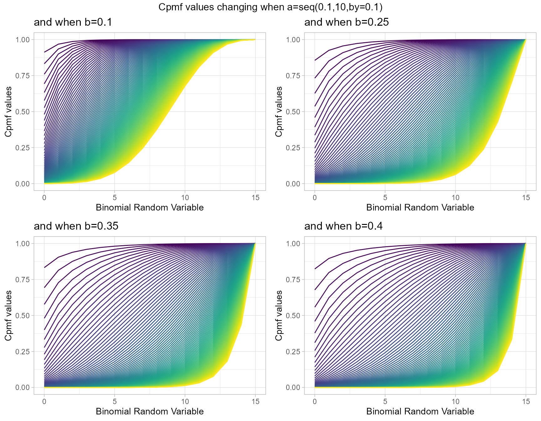
 a1 <- pGrassiaIIBinplot(b=seq(0.1,10,by=0.1),a=0.1,plot_title="and when a=0.1",a_seq= F)
a25 <- pGrassiaIIBinplot(b=seq(0.1,10,by=0.1),a=0.25,plot_title="and when a=0.25",a_seq= F)
 a5 <- pGrassiaIIBinplot(b=seq(0.1,10,by=0.1),a=0.5,plot_title="and when a=0.5",a_seq= F)
a10 <- pGrassiaIIBinplot(b=seq(0.1,10,by=0.1),a=1,plot_title="and when a=1",a_seq= F)

grid.arrange(a1,a25,a5,a10,nrow=2,top="Cpmf values changing when b=seq(0.1,10,by=0.1)")
Alternate Binomial Distributions
with the help of Pmf values Cpmf values are generated. At situations they have been very useful in replacing Binomial distributions. It can be understood by looking at the Cpmf values an its variety. Below are the functions which can produce Cpmf values
-
pAddBin- producing Cpmf values for Additive Binomial Distribution. -
pBetaCorrBin- producing Cpmf values for Beta-Correlated Binomial Distribution. -
pCOMPBin- producing Cpmf Values for COM Poisson Binomial Distribution. -
pCorrBin- producing Cpmf values for Correlated Binomial Distribution. -
pMultiBin- producing Cpmf values for Multiplicative Binomial Distribution. -
pLMBin- producing Cpmf values for Lovinson Multiplicative Binomial Distribution.
When there is more than one changing parameter in the distribution, there needs to be specific functions to plot the Cpmf values. Below given functions have the ability to do so
-
pAddBinplot- plot function to Additive Binomial Distribution. -
pBetaCorrBinplot- plot function to Beta Correlated Binomial Distribution. -
pCOMPBinplot- plot function to COM Poisson Binomial Distribution. -
pCorrBinplot- plot function to Correlated Binomial Distribution. -
pMultiBinplot- plot function to Multiplicative Binomial Distribution. -
pLMBinplot- plot function to Lovinson Multiplicative Binomial Distribution.
Cumulative Probability Mass Function values for Additive Binomial Distribution
Probability value and alpha parameter are unique values involved with this distribution. Slight changes in alpha and probability value can interest in very wide changes towards Cpmf values generated. Below is the plot which explains this situations.
- p value in-between zero and one.
- alpha value in-between negative one and positive one.
 alpha.001 <- pAddBinplot(p=seq(0.35,0.65,by=0.0001),alpha=-0.001,
                       plot_title="and when alpha=-0.001",p_seq= T)
 alpha.003 <- pAddBinplot(p=seq(0.35,0.65,by=0.0001),alpha=-0.003,
                       plot_title="and when alpha=-0.003",p_seq= T)
alpha0.005 <- pAddBinplot(p=seq(0.35,0.65,by=0.0001),alpha=0.005,
                        plot_title="and when alpha=0.005",p_seq= T)
alpha0.008 <- pAddBinplot(p=seq(0.35,0.65,by=0.0001),alpha=0.008,
                        plot_title="and when alpha=0.008",p_seq= T)

grid.arrange(alpha.001,alpha.003,alpha0.005,alpha0.008,nrow=2,
             top="Cpmf values changing when p=seq(0.35,0.65,by=0.0001)")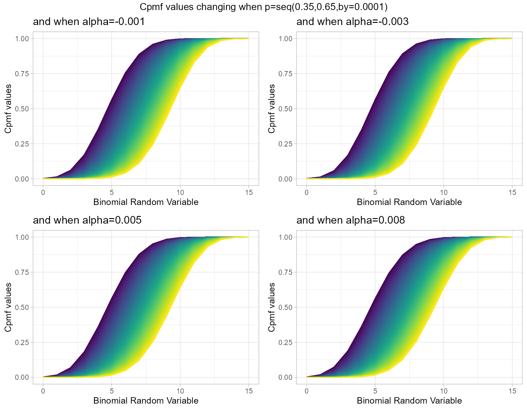
p.015 <- pAddBinplot(alpha=seq(0.0001,0.05,by=0.0001),p=0.015,
                  plot_title="and when p=0.0.15",p_seq= F)
p.115 <- pAddBinplot(alpha=seq(0.0001,0.05,by=0.0001),p=0.115,
                  plot_title="and when p=0.115",p_seq= F)
p.215 <- pAddBinplot(alpha=seq(0.0001,0.05,by=0.0001),p=0.215,
                  plot_title="and when p=0.215",p_seq= F)
p.315 <- pAddBinplot(alpha=seq(0.0001,0.05,by=0.0001),p=0.315,
                  plot_title="and when p=0.315",p_seq= F)

grid.arrange(p.015,p.115,p.215,p.315,nrow=2,
             top="Cpmf values changing when alpha=seq(0.0001,0.05,by=0.0001)")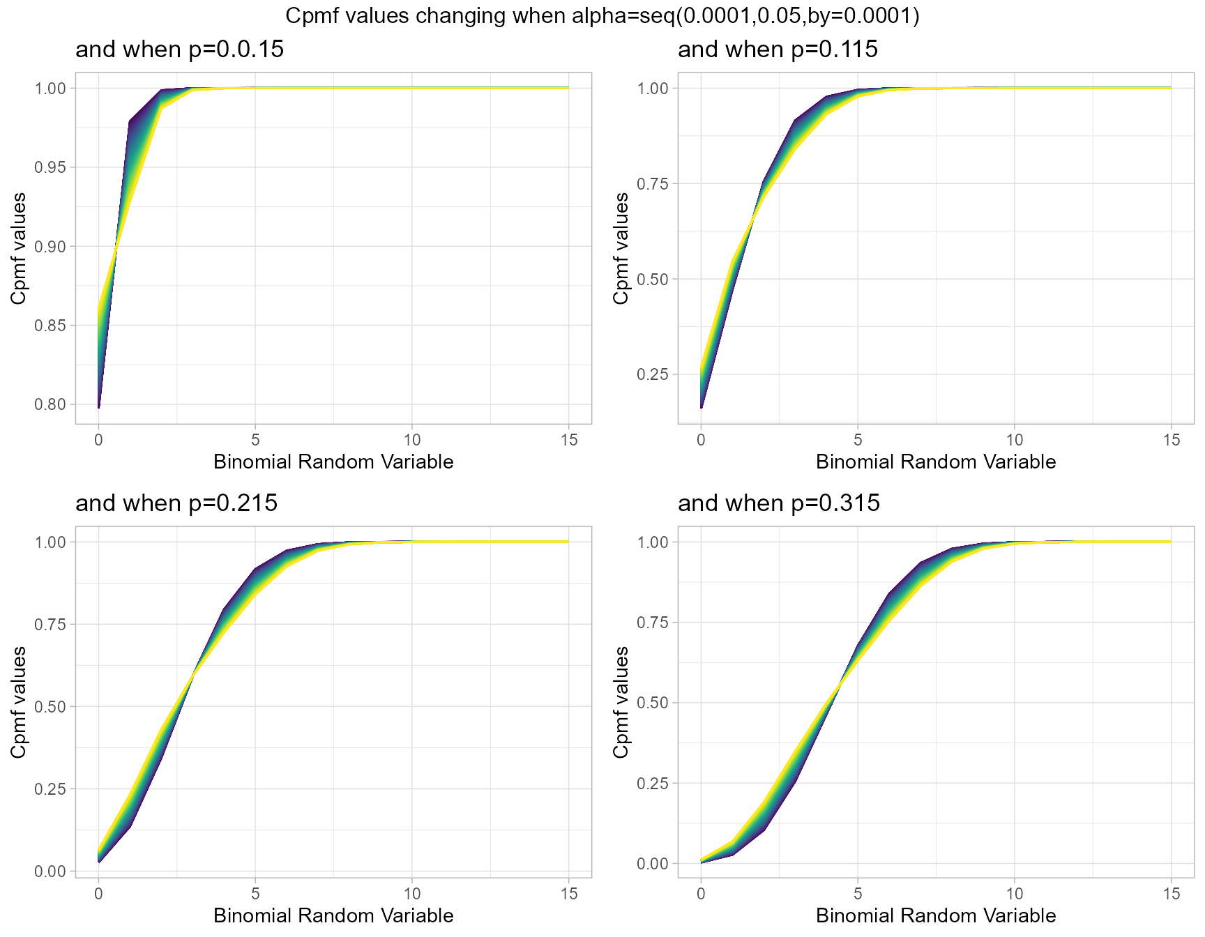
Cumulative Probability Mass Function values for Beta-Correlated Binomial Distribution
Three parameters are involved in producing Cpmf values for Beta-Correlated Binomial distribution. They are namely cov representing the covariance value from Correlated distribution and a,b are shape parameters from Beta distribution. Below is the plot describing how Cpmf values with related to cov, a and b parameters.
- cov is the covariance value in between negative infinity and positive infinity.
- a, b are in the domain region of above zero.
 b16cov5 <- pBetaCorrBinplot(a=seq(10,100,by=0.1),b=16,cov=0.0005,
                 plot_title="and when b=16, cov=0.0005",a_seq=T,b_seq=F)
 b46cov5 <- pBetaCorrBinplot(a=seq(10,100,by=0.1),b=46,cov=0.0005,
                   plot_title="and when b=46, cov=0.0005",a_seq=T,b_seq=F)
 b76cov5 <- pBetaCorrBinplot(a=seq(10,100,by=0.1),b=76,cov=0.0005,
                 plot_title="and when b=76, cov=0.0005",a_seq=T,b_seq=F)
b106cov5 <- pBetaCorrBinplot(a=seq(10,100,by=0.1),b=106,cov=0.0005,
                   plot_title="and when b=106 cov=0.0005",a_seq=T,b_seq=F)

grid.arrange(b16cov5,b46cov5,b76cov5,b106cov5,nrow=2,
             top="Cpmf values changing when a=seq(10,100,by=0.1)")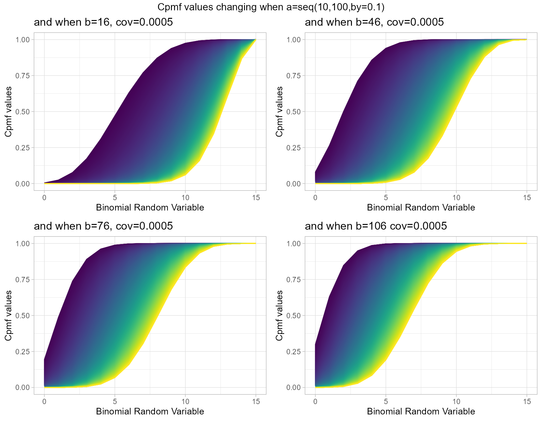
b10cov1 <- pBetaCorrBinplot(a=seq(15,100,by=0.1),b=10,cov=0.001,
                 plot_title="and when b=10, cov=0.001",a_seq=T,b_seq=F)
b10cov3 <- pBetaCorrBinplot(a=seq(15,100,by=0.1),b=10,cov=0.003,
                   plot_title="and when b=10, cov=0.003",a_seq=T,b_seq=F)
b10cov7 <- pBetaCorrBinplot(a=seq(15,100,by=0.1),b=10,cov=0.007,
                 plot_title="and when b=10, cov=0.007",a_seq=T,b_seq=F)
b10cov9 <- pBetaCorrBinplot(a=seq(15,100,by=0.1),b=10,cov=0.009,
                   plot_title="and when b=10, cov=0.009",a_seq=T,b_seq=F)

grid.arrange(b10cov1,b10cov3,b10cov7,b10cov9,nrow=2,
             top="Cpmf values changing when a=seq(15,100,by=0.1)")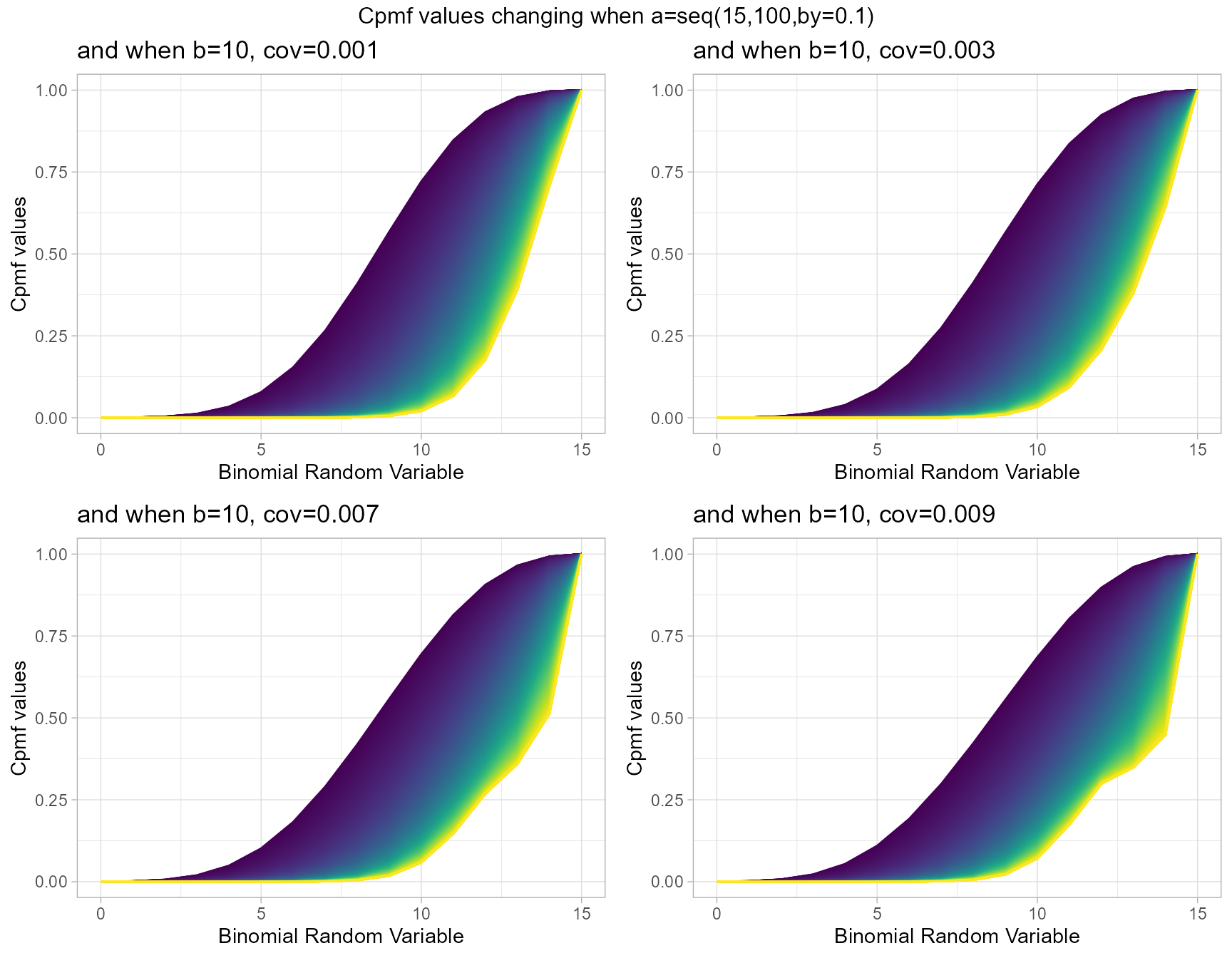
Cumulative Probability Mass Function values for COM Poisson Binomial Distribution
COM Poisson Binomial distribution has two parameters in concern which are probability value and covariance value. Considering the covariance is very special and useful as it can explain the over-dispersion. Below is the plot explaining this situation
- p is the probability value in between zero and one.
- v is the covariance value in between negative infinity and positive infinity.
v.5 <- pCOMPBinplot(p=seq(0.25,0.75,by=0.001),v=0.5,
                   plot_title="and when v=0.5",p_seq= T)
 v1 <- pCOMPBinplot(p=seq(0.25,0.75,by=0.001),v=1,
                   plot_title="and when v=1",p_seq= T)
 v3 <- pCOMPBinplot(p=seq(0.25,0.75,by=0.001),v=3,
                   plot_title="and when v=3",p_seq= T)
 v5 <- pCOMPBinplot(p=seq(0.25,0.75,by=0.001),v=5,
                   plot_title="and when v=5",p_seq= T)

grid.arrange(v.5,v1,v3,v5,nrow=2,
             top="Cpmf values changing when p=seq(0.25,0.75,by=0.001)")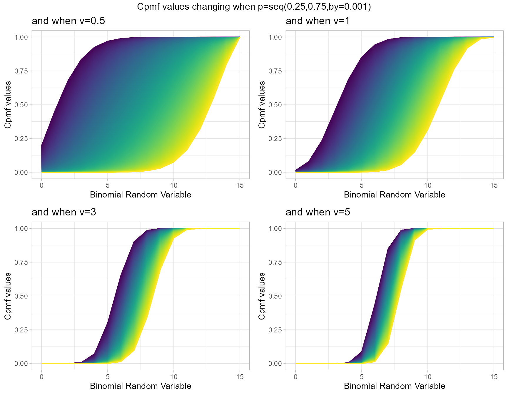
p0.40 <- pCOMPBinplot(v=seq(-0.5,5.5,by=.01),p=0.40,
                    plot_title="and when p=0.35",p_seq= F)
p0.45 <- pCOMPBinplot(v=seq(-0.5,5.5,by=.01),p=0.45,
                    plot_title="and when p=0.45",p_seq= F)
p0.50 <- pCOMPBinplot(v=seq(-0.5,5.5,by=.01),p=0.50,
                    plot_title="and when p=0.55",p_seq= F)
p0.55 <- pCOMPBinplot(v=seq(-0.5,5.5,by=.01),p=0.55,
                    plot_title="and when p=0.65",p_seq= F)

grid.arrange(p0.40,p0.45,p0.50,p0.55,nrow=2,
             top="Cpmf values changing when v=seq(-0.5,5.5,by=0.01)")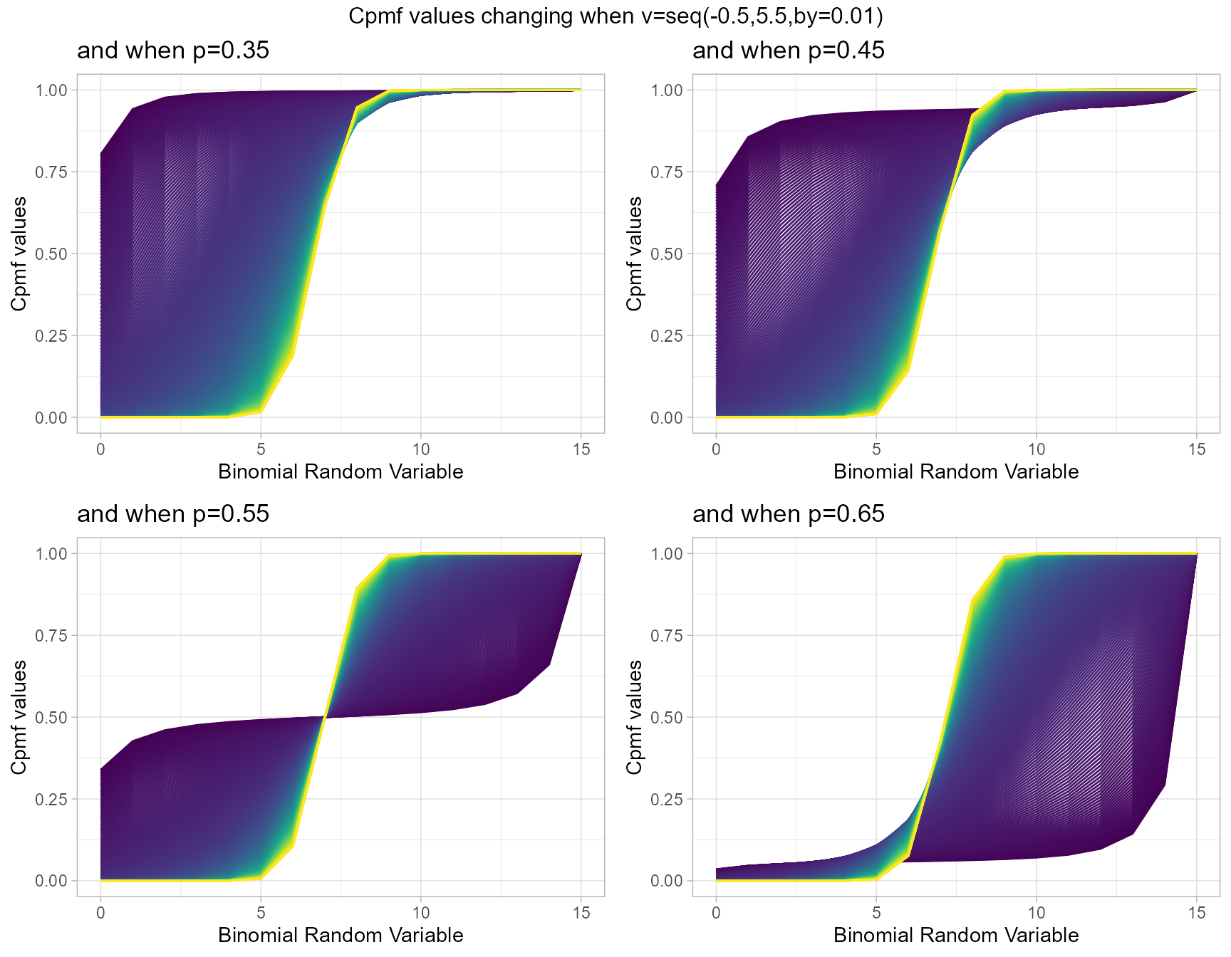
Cumulative Probability Mass Function values for Correlated Binomial Distribution
Correlated Binomial distribution simply considers the correlation among binary trials, which can result in over-dispersion. Rather than this the probability value is also a part of this distribution. When ever covariance and probability value change the Cpmf values also change. Below is a simple plot elaborating that.
- p is the probability value in between zero and one.
- cov is the covariance value in between negative infinity and positive infinity.
 cov0.001 <- pCorrBinplot(p=seq(0.15,0.75,by=0.01),cov=0.001,
                        plot_title="and when cov=0.001",p_seq= T)
 cov0.004 <- pCorrBinplot(p=seq(0.15,0.75,by=0.01),cov=0.004,
                        plot_title="and when cov=0.004",p_seq= T)
 cov0.005 <- pCorrBinplot(p=seq(0.15,0.75,by=0.01),cov=0.005,
                        plot_title="and when cov=0.005",p_seq= T)
  cov0.01 <- pCorrBinplot(p=seq(0.15,0.75,by=0.01),cov=0.01,
                        plot_title="and when cov=0.01",p_seq= T)

grid.arrange(cov0.001,cov0.004,cov0.005,cov0.01,nrow=2,
             top="Cpmf values changing when p=seq(0.15,0.75,by=0.01)")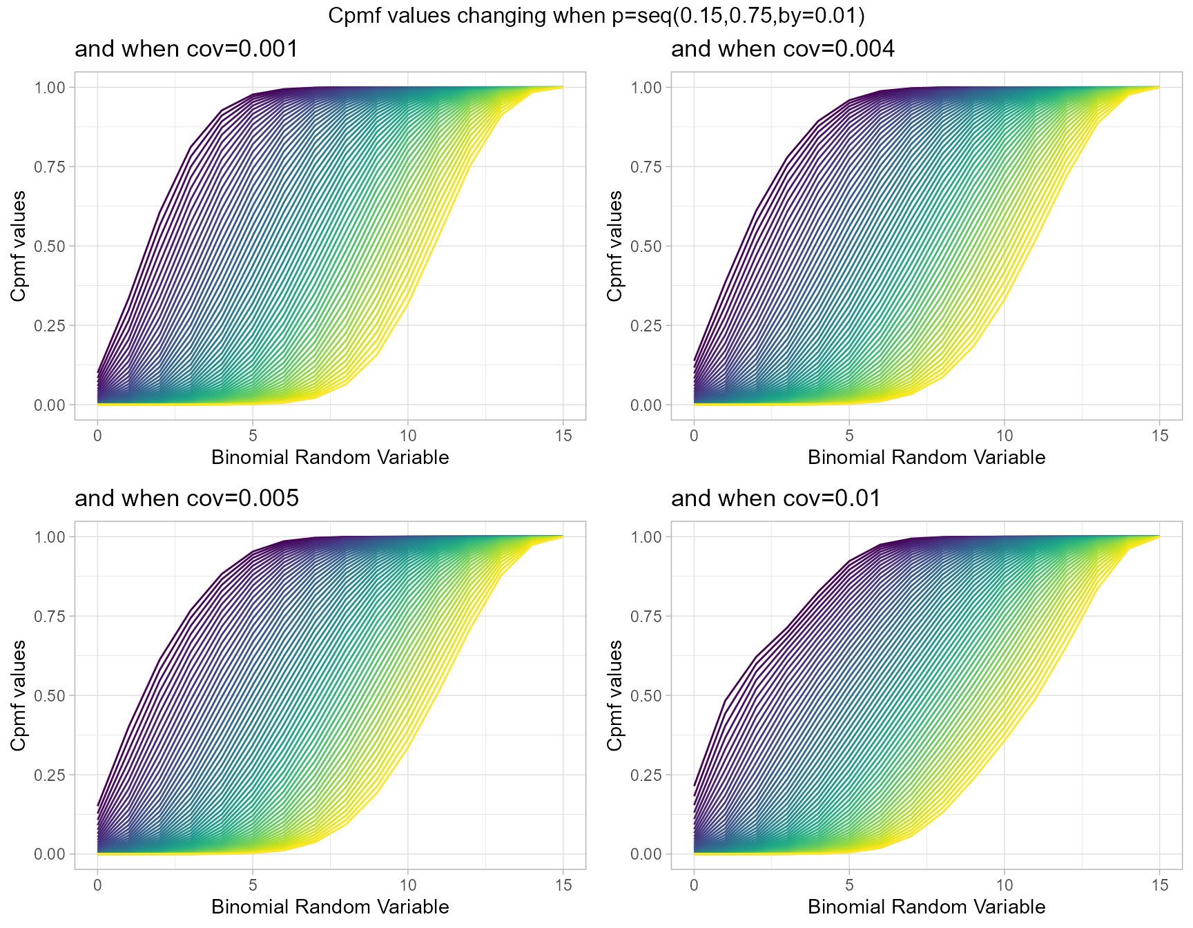
p0.15 <- pCorrBinplot(cov=seq(0.002,0.009,by=.0001),p=0.15,
                    plot_title="and when p=0.15",p_seq= F)
p0.25 <- pCorrBinplot(cov=seq(0.002,0.009,by=.0001),p=0.25,
                    plot_title="and when p=0.25",p_seq= F)
p0.50 <- pCorrBinplot(cov=seq(0.002,0.009,by=.0001),p=0.50,
                    plot_title="and when p=0.50",p_seq= F)
p0.75 <- pCorrBinplot(cov=seq(0.002,0.009,by=.0001),p=0.75,
                    plot_title="and when p=0.75",p_seq= F)

grid.arrange(p0.15,p0.25,p0.50,p0.75,nrow=2,
             top="Cpmf values changing when cov=seq(0.002,0.009,by=0.0001)")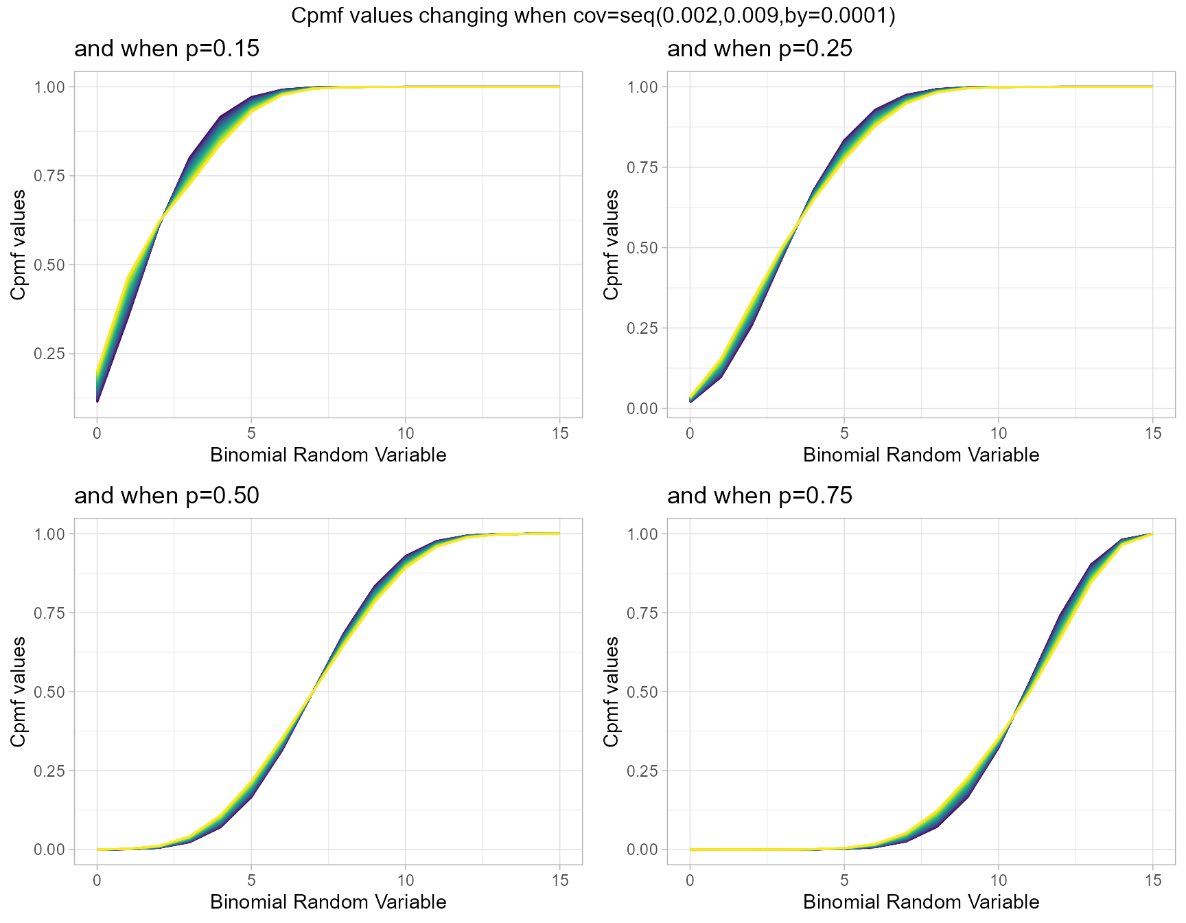
Cumulative Probability Mass Function values for Multiplicative Binomial Distribution
Multiplicative Binomial Distribution also has two important parameters they are probability value p and theta parameter. Given below are the plots describing how Cpmf values change with respective to p and theta.
- p is the probability value in between zero and one.
- theta parameter is in the domain region of above zero.
   theta1 <- pMultiBinplot(p=seq(0.01,0.99,by=0.005),theta=1,
                       plot_title="and when theta=1",p_seq= T)
theta1.25 <- pMultiBinplot(p=seq(0.01,0.99,by=0.005),theta=1.25,
                       plot_title="and when theta=1.25",p_seq= T)
theta1.75 <- pMultiBinplot(p=seq(0.01,0.99,by=0.005),theta=1.75,
                      plot_title="and when theta=1.75",p_seq= T)
   theta2 <- pMultiBinplot(p=seq(0.01,0.99,by=0.005),theta=2,
                      plot_title="and when theta=2",p_seq= T)

grid.arrange(theta1,theta1.25,theta1.75,theta2,nrow=2,
             top="Cpmf values changing when p=seq(0.01,0.99,by=0.005)")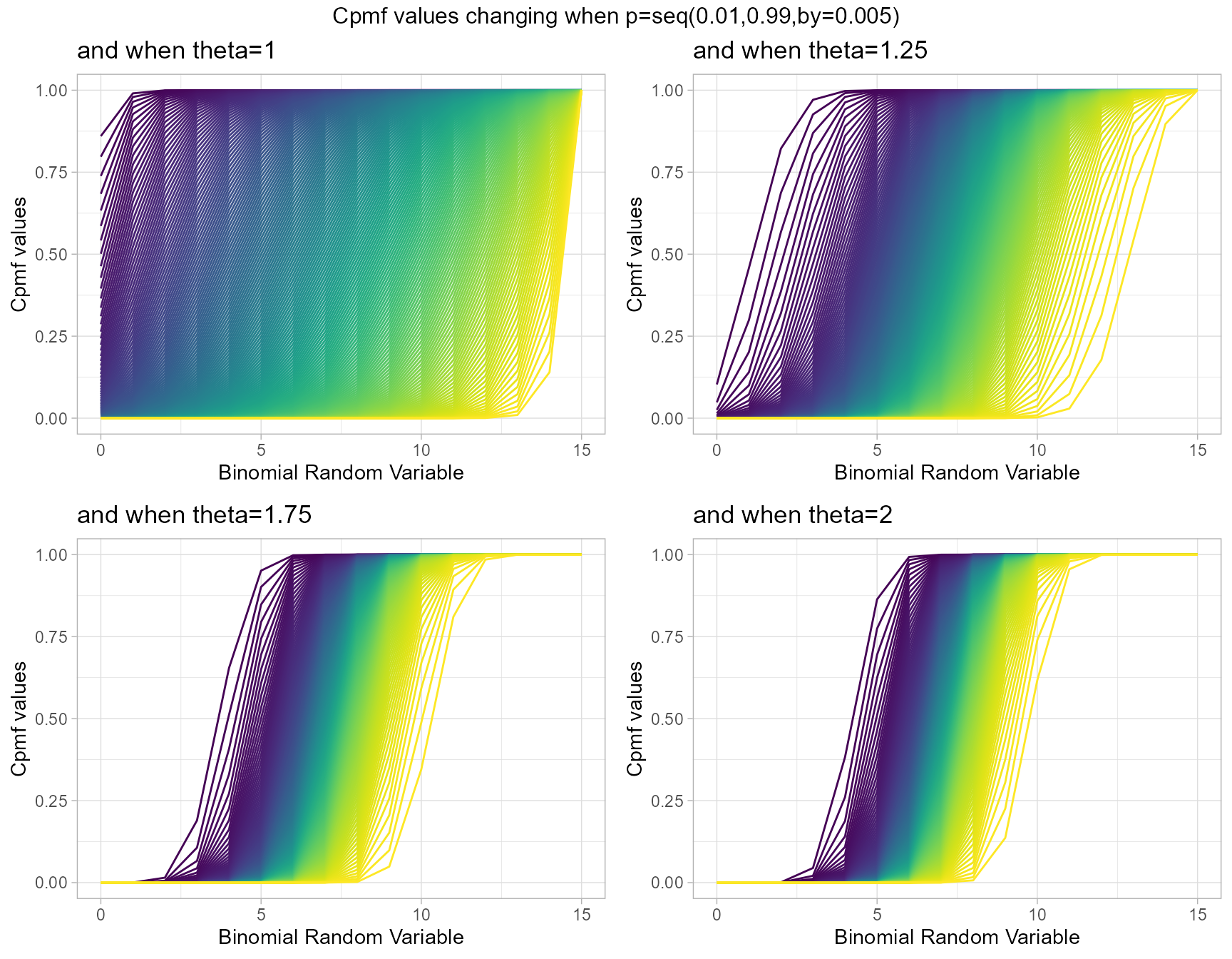
p0.35 <- pMultiBinplot(theta=seq(1.001,5,by=0.001),p=0.35,
                     plot_title="and when p=0.35",p_seq= F)
p0.45 <- pMultiBinplot(theta=seq(1.001,5,by=0.001),p=0.45,
                     plot_title="and when p=0.45",p_seq= F)
p0.55 <- pMultiBinplot(theta=seq(1.001,5,by=0.001),p=0.55,
                     plot_title="and when p=0.55",p_seq= F)
p0.65 <- pMultiBinplot(theta=seq(1.001,5,by=0.001),p=0.65,
                     plot_title="and when p=0.65",p_seq= F)

grid.arrange(p0.35,p0.45,p0.55,p0.65,nrow=2,
             top="Cpmf values changing when theta=seq(1.001,5,by=0.001)")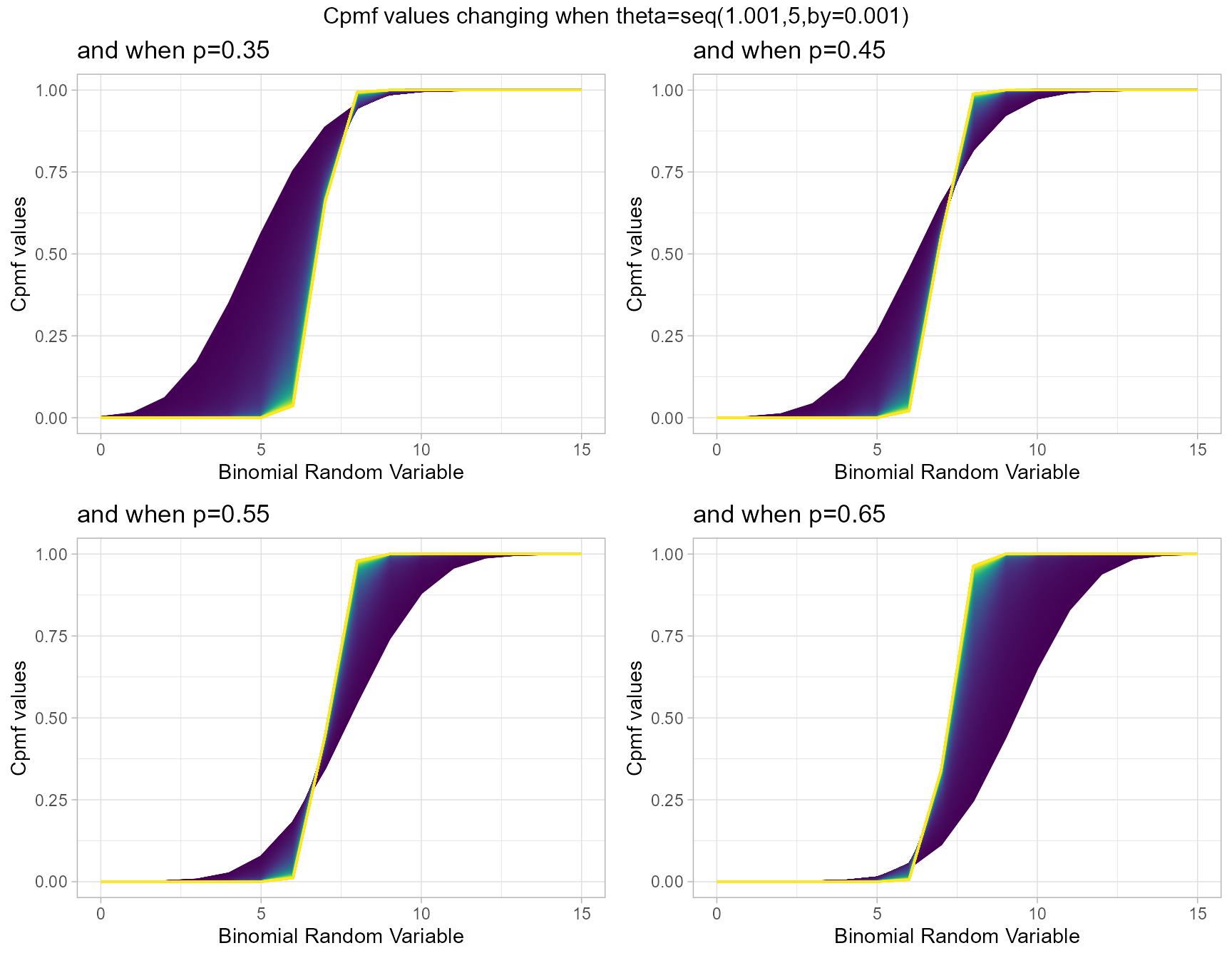
Cumulative Probability Mass Function values for Lovinson Multiplicative Binomial Distribution
Lovinson Multiplicative Binomial Distribution also has two important parameters they are probability value p and phi parameter. Given below are the plots describing how Cpmf values change with respective to p and phi.
- p is the probability value in between zero and one.
- phi parameter is in the domain region of above zero.
   phi1 <- pLMBinplot(p=seq(0.01,0.99,by=0.001),phi=1,
                      plot_title="and when phi=1",p_seq= T)
phi1.25 <- pLMBinplot(p=seq(0.01,0.99,by=0.001),phi=1.25,
                         plot_title="and when phi=1.25",p_seq= T)
phi1.75 <- pLMBinplot(p=seq(0.01,0.99,by=0.001),phi=1.75,
                         plot_title="and when phi=1.75",p_seq= T)
   phi2 <- pLMBinplot(p=seq(0.01,0.99,by=0.001),phi=2,
                      plot_title="and when phi=2",p_seq= T)

grid.arrange(phi1,phi1.25,phi1.75,phi2,nrow=2,
             top="Cpmf values changing when p=seq(0.01,0.99,by=0.001)")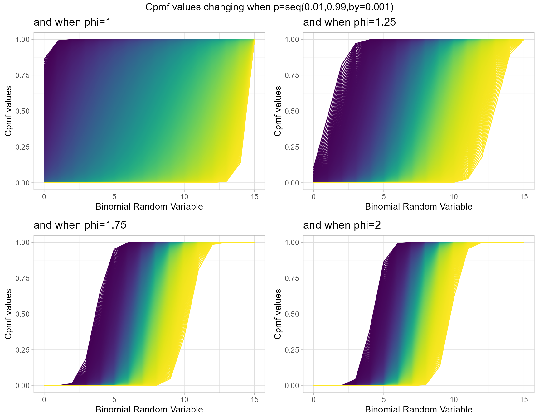
p0.35 <- pLMBinplot(phi=seq(1.001,5,by=0.001),p=0.35,
                     plot_title="and when p=0.35",p_seq= F)
p0.45 <- pLMBinplot(phi=seq(1.001,5,by=0.001),p=0.45,
                     plot_title="and when p=0.45",p_seq= F)
p0.55 <- pLMBinplot(phi=seq(1.001,5,by=0.001),p=0.55,
                     plot_title="and when p=0.55",p_seq= F)
p0.65 <- pLMBinplot(phi=seq(1.001,5,by=0.001),p=0.65,
                     plot_title="and when p=0.65",p_seq= F)

grid.arrange(p0.35,p0.45,p0.55,p0.65,nrow=2,
             top="Cpmf values changing when phi=seq(1.001,5,by=0.001)")