These functions provide the ability for generating probability function values and cumulative probability function values for the Gamma Binomial Distribution.
pGammaBin(x,n,c,l)
Arguments
| x | vector of binomial random variables. |
|---|---|
| n | single value for no of binomial trials. |
| c | single value for shape parameter c. |
| l | single value for shape parameter l. |
Value
The output of pGammaBin gives cumulative probability values in vector form.
Details
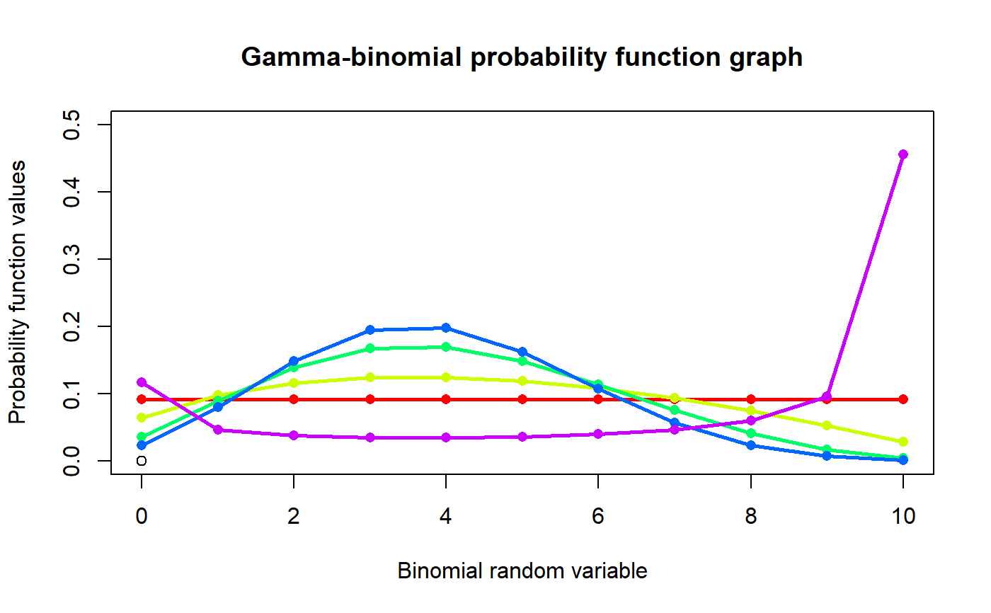
Mixing Gamma distribution with Binomial distribution will create the the Gamma Binomial distribution. The probability function and cumulative probability function can be constructed and are denoted below.
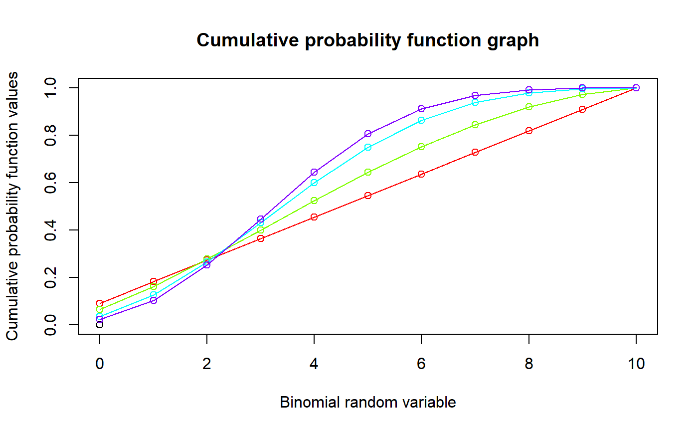
The cumulative probability function is the summation of probability function values.
$$P_{GammaBin}[x]= {n \choose x} \sum_{j=0}^{n-x} {n-x \choose j} (-1)^j (\frac{c}{c+x+j})^l $$ $$c,l > 0$$ $$x = 0,1,2,...,n$$ $$n = 1,2,3,...$$
The mean, variance and over dispersion are denoted as $$E_{GammaBin}[x] = (\frac{c}{c+1})^l$$ $$Var_{GammaBin}[x] = n^2[(\frac{c}{c+2})^l - (\frac{c}{c+1})^{2l}] + n(\frac{c}{c+1})^l{1-)(\frac{c+1}{c+2})^l}$$ $$over dispersion= \frac{(\frac{c}{c+2})^l - (\frac{c}{c+1})^{2l}}{(\frac{c}{c+1})^l[1-(\frac{c}{c+1})^l]}$$
References
Grassia, A., 1977. On a family of distributions with argument between 0 and 1 obtained by transformation of the gamma and derived compound distributions. Australian Journal of Statistics, 19(2), pp.108-114.
Examples
#plotting the random variables and probability values col <- rainbow(5) a <- c(1,2,5,10,0.2) plot(0,0,main="Gamma-binomial probability function graph",xlab="Binomial random variable", ylab="Probability function values",xlim = c(0,10),ylim = c(0,0.5))for (i in 1:5) { lines(0:10,dGammaBin(0:10,10,a[i],a[i])$pdf,col = col[i],lwd=2.85) points(0:10,dGammaBin(0:10,10,a[i],a[i])$pdf,col = col[i],pch=16) }#> [1] 5.870615e-05 2.754357e-04 8.057584e-04 1.892811e-03 3.928276e-03 #> [6] 7.579979e-03 1.409128e-02 2.611031e-02 5.066078e-02 1.162261e-01 #> [11] 7.783705e-01#> [1] 9.563525#> [1] 1.092227#> [1] 0.1796209#plotting the random variables and cumulative probability values col <- rainbow(4) a <- c(1,2,5,10) plot(0,0,main="Cumulative probability function graph",xlab="Binomial random variable", ylab="Cumulative probability function values",xlim = c(0,10),ylim = c(0,1))for (i in 1:4) { lines(0:10,pGammaBin(0:10,10,a[i],a[i]),col = col[i]) points(0:10,pGammaBin(0:10,10,a[i],a[i]),col = col[i]) }pGammaBin(0:10,10,4,.2) #acquiring the cumulative probability values#> [1] 5.870615e-05 3.341419e-04 1.139900e-03 3.032711e-03 6.960987e-03 #> [6] 1.454097e-02 2.863224e-02 5.474255e-02 1.054033e-01 2.216295e-01 #> [11] 1.000000e+00