IT WOULD BE CLEARLY BENEFICIAL FOR YOU BY USING THE RMD FILES IN THE GITHUB DIRECTORY FOR FURTHER EXPLANATION OR UNDERSTANDING OF THE R CODE FOR THE RESULTS OBTAINED IN THE VIGNETTES.

Binomial Mixture Distributions

Binomial Mixture Distributions are developed for the purpose of fitting over dispersed Binomial outcome data. When Binomial Distribution and its conditions are violated the Binomial Mixture Distributions play a crucial role in fitting the data.

Here, we will be using plotting of Probability Mass Function values to understand how much variation can the probabilities have with the Binomial Mixture Distributions. These distributions are theoretically developed by mixing Unit Bounded distributions with the Binomial Distribution. The functions which can produce Pmf values for Binomial Mixture distributions are

dUniBin - producing Pmf values primarily for Uniform Binomial Distribution.
dTriBin - producing Pmf values primarily for Triangular Binomial Distribution.
dBetaBin - producing Pmf values primarily for Beta-Binomial Distribution.
dKumBin - producing Pmf values primarily for Kumaraswamy Binomial Distribution.
dGHGBB - producing Pmf values primarily for Gaussian Hyper-geometric Generalized Beta-Binomial Distribution.
dMcGBB - producing Pmf values primarily for McDonald Generalized Beta-Binomial Distribution.
dGammaBin - producing Pmf values primarily for Gamma Binomial Distribution.
dGrassiaIIBin - producing Pmf values primarily for Grassia II Binomial Distribution.

When the no of shape parameters increase plotting variation of pmf values is difficult therefore special Pmf plot functions are developed. They are namely

dBetaBinplot - plot function to Beta-Binomial Distribution.
dKumBinplot - plot function to Kumaraswamy Binomial Distribution.
dGHGBBplot - plot function to Gaussian Hyper-geometric Generalized Beta-Binomial Distribution.
dMcGBBplot - plot function to McDonald Generalized Beta-Binomial Distribution.
dGammaBinplot - plot function to Gamma Binomial Distribution.
dGrassiaIIBinplot - plot function Grassia II Binomial Distribution.

Probability Mass Function values for Uniform Binomial Distribution

Uniform Binomial distribution is the earliest development with least amount of over dispersed Binomial Random variables. There is no shape parameter which make this distribution very limited. Below is the of pmf values

brv <- 0:10
pmfv <- dUniBin(brv,max(brv))$pdf
data <- data.frame(brv,pmfv)
ggplot(data)+
  geom_point(aes(x=data$brv,y=data$pmfv))+
  geom_line(aes(x=data$brv,y=data$pmfv))+
  xlab("Binomial Random Variables")+
  ylab("Probability Mass Function values")+
  ggtitle("Pmf values changing")+
  ggthemes::theme_clean()+
  scale_x_continuous(breaks=seq(0,10,by=1))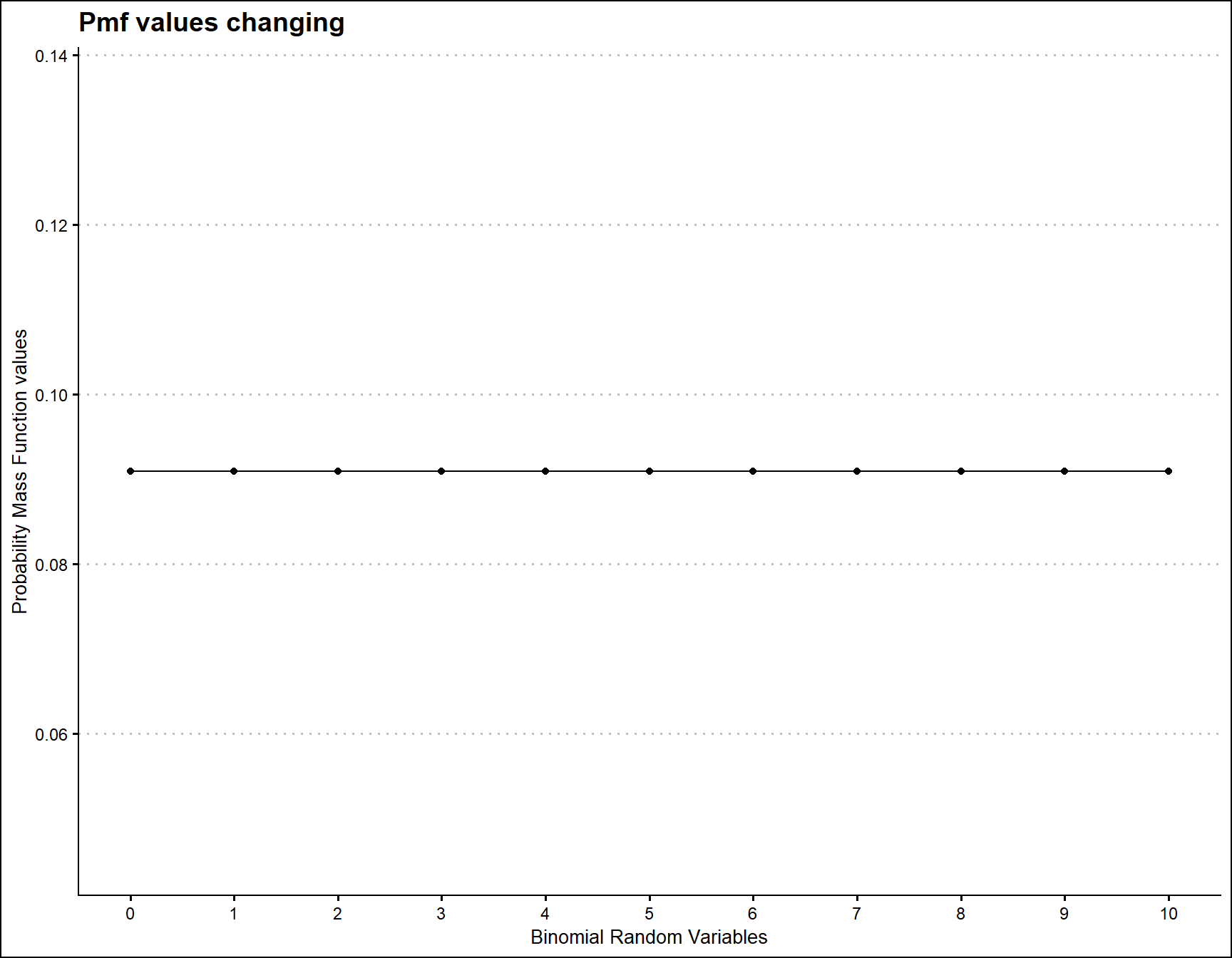

Probability Mass Function values for Triangular Binomial Distribution

Triangular Binomial Distribution has one parameter which has immense effect on the pmf values. Which is the mode parameter in the domain region of zero and one. According to the changes made in mode parameter pmf values will react and it has been plotted below

brv <- seq(0,15,by=1)
mode <- seq(0.02,0.98,by=0.02)
length(mode) #variables

## [1] 49

output <- matrix(ncol =length(mode) ,nrow=length(brv))
for (i in 1:length(mode)) 
  {
   output[,i]<-dTriBin(brv,max(brv),mode[i])$pdf
  }
data <- data.frame(brv,output)
data <- melt(data,id.vars ="brv" )
ggplot(data,aes(brv,value,col=variable))+
  geom_line()+guides(fill=FALSE,color=FALSE)+
  xlab("Binomial Random Variable")+
  ylab("Probability Mass values")+
  ggthemes::theme_clean()+
  ggtitle("Triangular Binomial Distribution using dTriBin function")+
  scale_x_continuous(breaks=seq(0,15,by=1))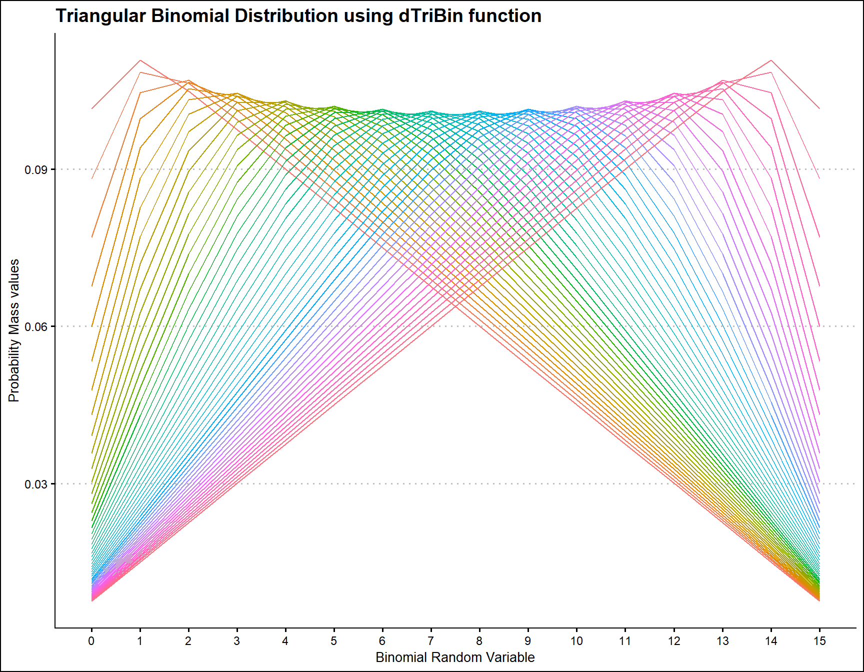

Probability Mass Function values for Beta-Binomial Distribution

Beta-Binomial Distribution has two shape parameters which influence the pmf values. They are namely a and b. These two parameters are inherited from the Beta distribution when mixing it to the Binomial Distribution. Pmf values are plotted below according to a and b values change

a,b are in the domain region of above zero.

 b10 <- dBetaBinplot(a=seq(1,100,by=1),b=10,plot_title="and when b=10",a_seq= T)
 b50 <- dBetaBinplot(a=seq(1,100,by=1),b=50,plot_title="and when b=50",a_seq= T)
b100 <- dBetaBinplot(a=seq(1,100,by=1),b=100,plot_title="and when b=100",a_seq= T)
b200 <- dBetaBinplot(a=seq(1,100,by=1),b=200,plot_title="and when b=200",a_seq= T)

grid.arrange(b10,b50,b100,b200,nrow=2,top="Pmf values changing when a=seq(1,100,by=1)")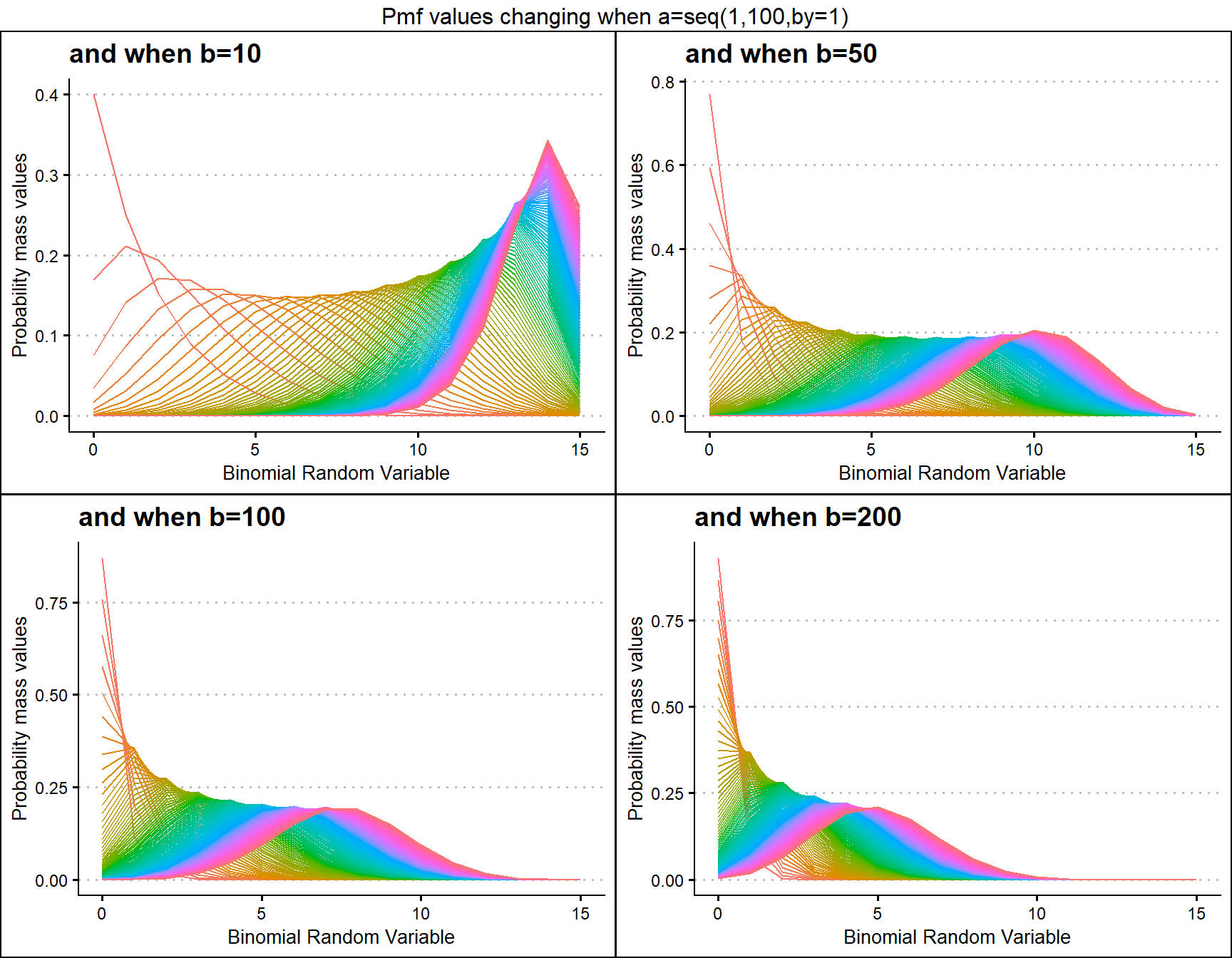

 a10 <- dBetaBinplot(b=seq(1,100,by=1),a=10,plot_title="and when a=10",a_seq= F)
 a50 <- dBetaBinplot(b=seq(1,100,by=1),a=50,plot_title="and when a=50",a_seq= F)
a100 <- dBetaBinplot(b=seq(1,100,by=1),a=100,plot_title="and when a=100",a_seq= F)
a200 <- dBetaBinplot(b=seq(1,100,by=1),a=200,plot_title="and when a=200",a_seq= F)

grid.arrange(a10,a50,a100,a200,nrow=2,top="Pmf values changing when b=seq(1,100,by=1)")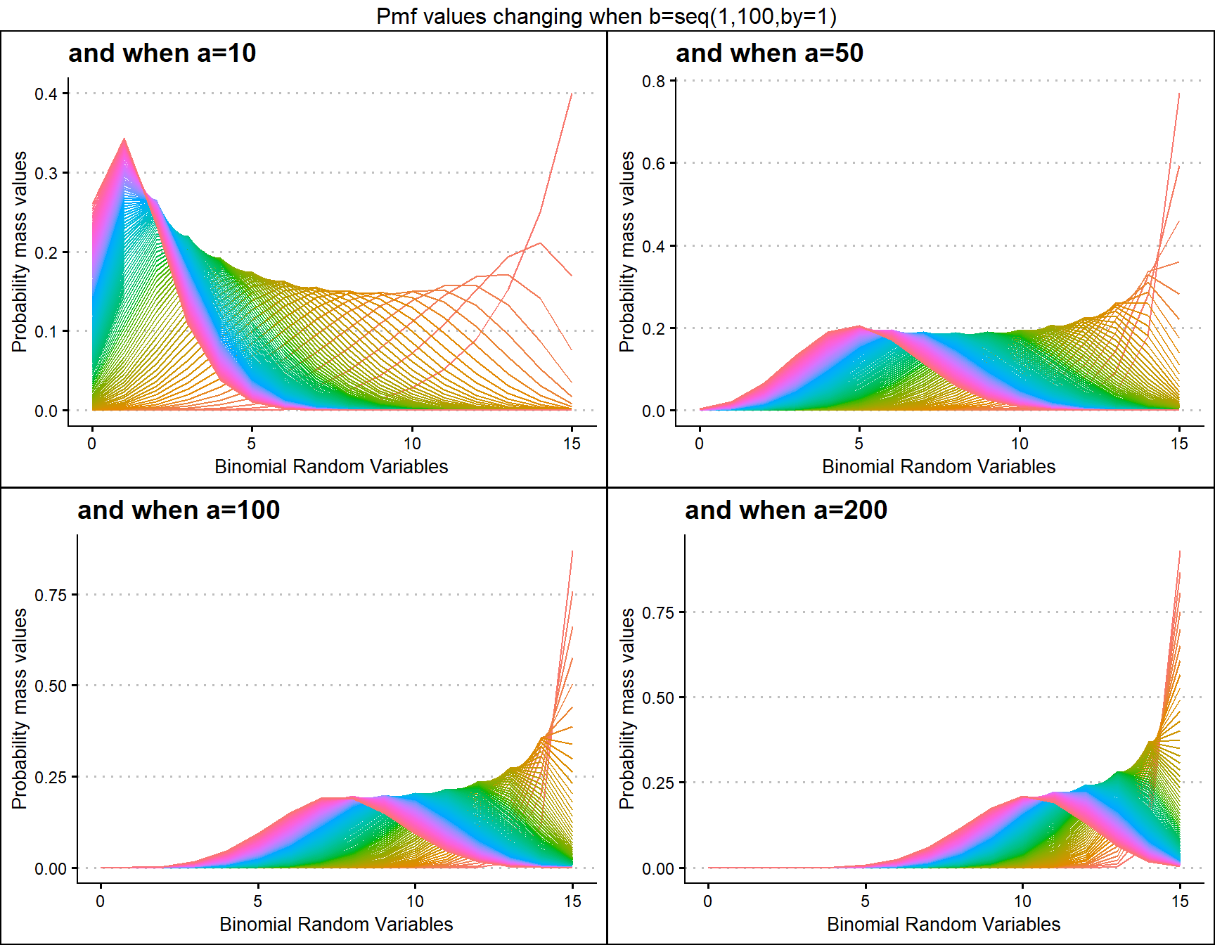

Probability Mass Function values for Kumaraswamy Binomial Distribution

Kumaraswamy Binomial distribution is similar to Beta-Binomial distribution with two shape parameters. Mixing Kumaraswamy distribution with Binomial distribution results in Kumaraswamy Binomial Distribution. The two shape parameters are a and b. Below are the plots for describing how pmf values change with respective to those a and b shape parameters.

a,b are in the domain region of above zero.
iteration parameter replacing the infinity value in the summation part.

 b5 <- dKumBinplot(a=seq(1,50,by=1),b=5,plot_title="and when b=5",a_seq=T)
b10 <- dKumBinplot(a=seq(1,50,by=1),b=10,plot_title="and when b=10",a_seq=T)
b20 <- dKumBinplot(a=seq(1,50,by=1),b=20,plot_title="and when b=20",a_seq=T)
b25 <- dKumBinplot(a=seq(1,50,by=1),b=25,plot_title="and when b=25",a_seq=T)

grid.arrange(b5,b10,b20,b25,nrow=2,top="Pmf values changing when a=seq(1,50,by=1)")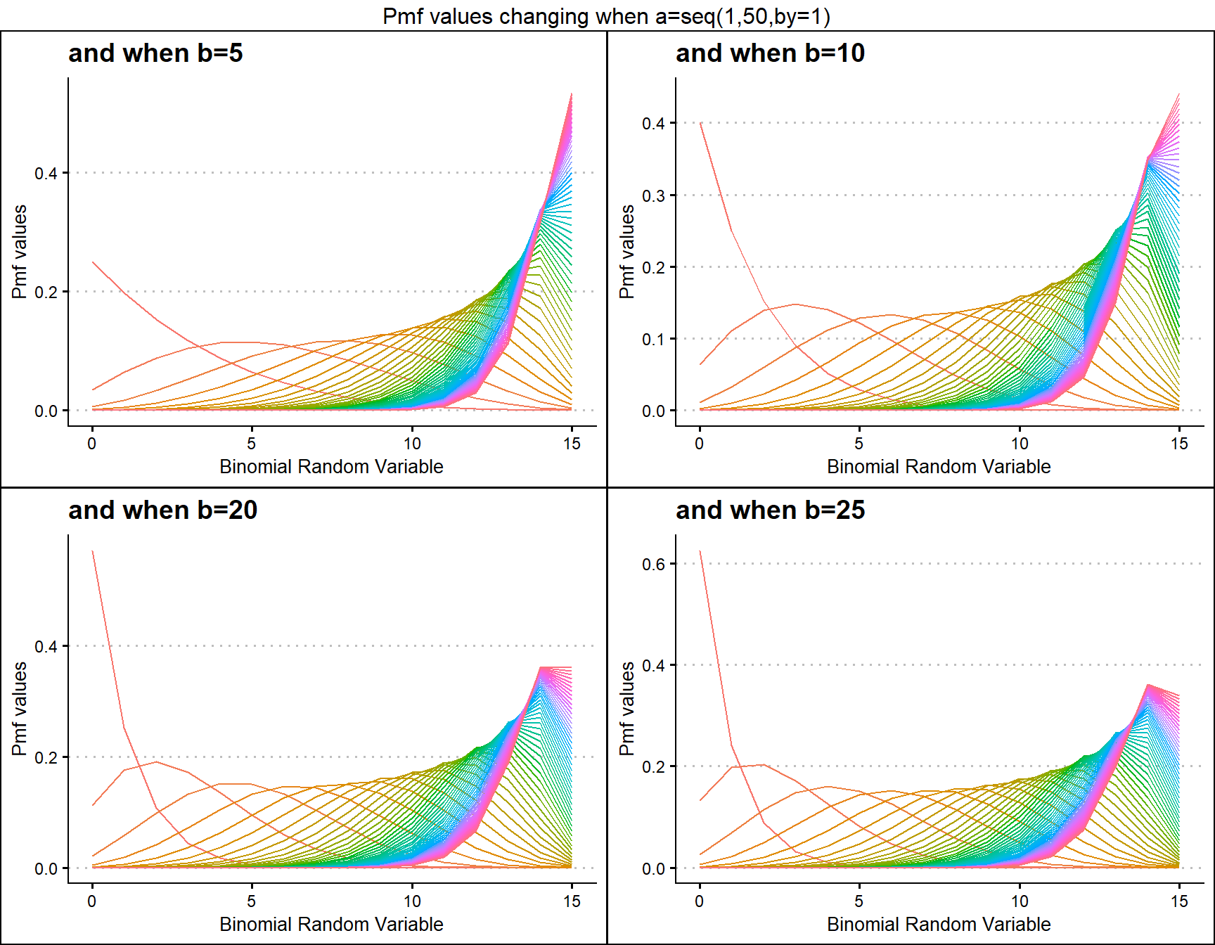

 a5 <- dKumBinplot(b=seq(1,30,by=1),a=5,plot_title="and when a=5",a_seq=F)
a10 <- dKumBinplot(b=seq(1,30,by=1),a=10,plot_title="and when a=10",a_seq=F)
a20 <- dKumBinplot(b=seq(1,30,by=1),a=20,plot_title="and when a=20",a_seq=F)
a25 <- dKumBinplot(b=seq(1,30,by=1),a=25,plot_title="and when a=25",a_seq=F)

grid.arrange(a5,a10,a20,a25,nrow=2,top="Pmf values changing when b=seq(1,30,by=1)")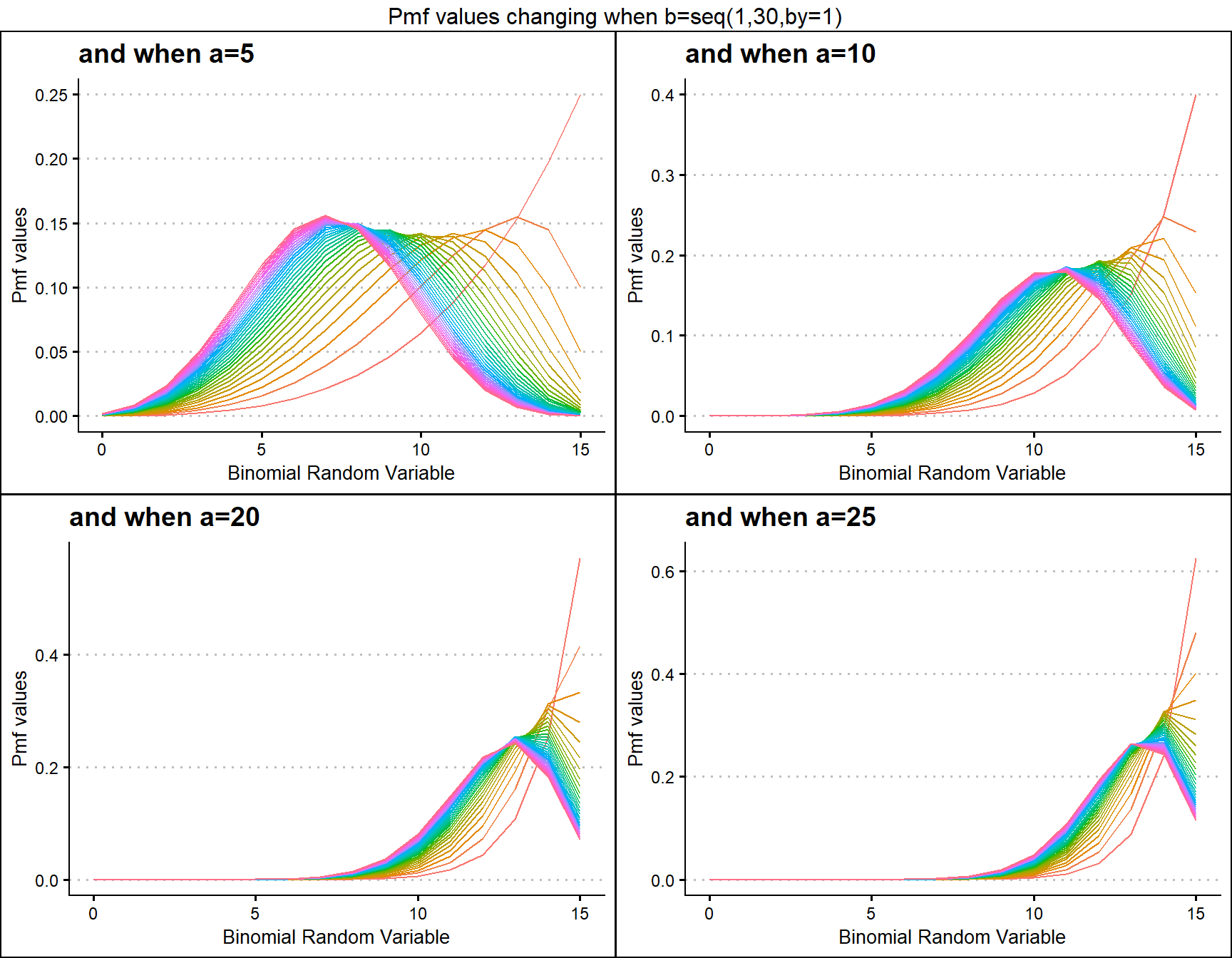

Probability Mass Function values for Gaussian Hyper-geometric Generalized Beta-Binomial Distribution

Gaussian Hyper-geometric Generalized Beta-Binomial or GHGBB distribution three shape parameters which influence the pmf values. They are a,b and c. The Gaussian hyper-geometric function plays a huge role in producing pmf values. To study about this function refer the package hypergeo. Having three parameters makes plotting pmf values more difficult still they provide more variation. Below is the plot for pmf values with respective to change in shape parameters.

a,b,c are in the domain region of above zero.

 b10c5 <- dGHGBBplot(a=seq(.1,100,by=.1),b=10,c=5,
                  plot_title="and when b=10, c=5",a_seq=T,b_seq=F)
 b50c5 <- dGHGBBplot(a=seq(.1,100,by=.1),b=50,c=5,
                  plot_title="and when b=50, c=5",a_seq=T,b_seq=F)
b100c5 <- dGHGBBplot(a=seq(.1,100,by=.1),b=100,c=5,
                   plot_title="and when b=100, c=5",a_seq=T,b_seq=F)
b200c5 <- dGHGBBplot(a=seq(.1,100,by=.1),b=150,c=5,
                   plot_title="and when b=200, c=5",a_seq=T,b_seq=F)

grid.arrange(b10c5,b50c5,b100c5,b200c5,nrow=2,
             top="Pmf values changing when a=seq(0.1,100,by=0.1)")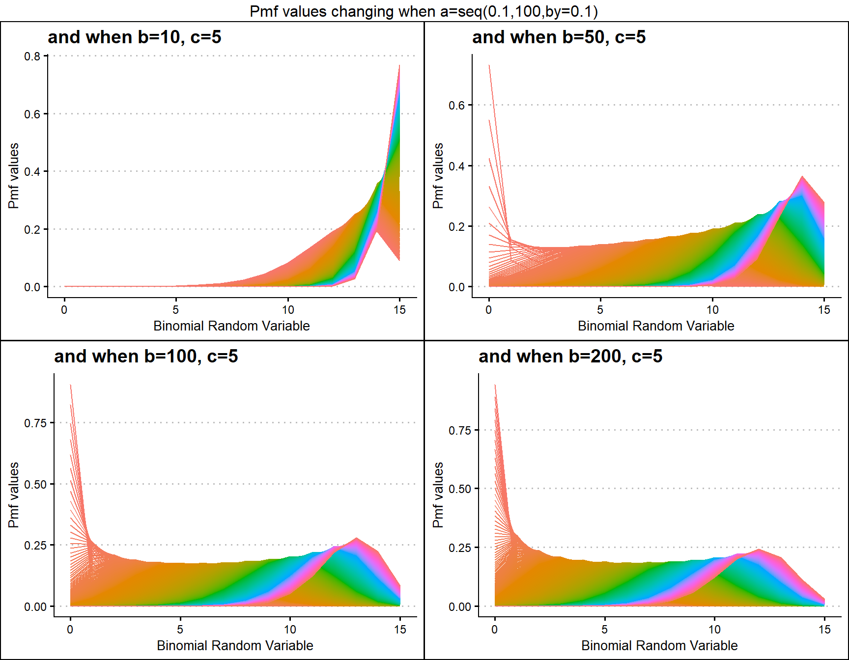

 b20c10 <- dGHGBBplot(a=seq(.1,100,by=.1),b=20,c=10,
                   plot_title="and when b=20, c=10",a_seq=T,b_seq=F)
 b50c10 <- dGHGBBplot(a=seq(.1,100,by=.1),b=50,c=10,
                   plot_title="and when b=50, c=10",a_seq=T,b_seq=F)
b100c10 <- dGHGBBplot(a=seq(.1,100,by=.1),b=100,c=10,
                    plot_title="and when b=100, c=10",a_seq=T,b_seq=F)
b200c10 <- dGHGBBplot(a=seq(.1,100,by=.1),b=200,c=10,
                    plot_title="and when b=200, c=10",a_seq=T,b_seq=F)

grid.arrange(b20c10,b50c10,b100c10,b200c10,nrow=2,
             top="Pmf values changing when a=seq(0.1,100,by=0.1)")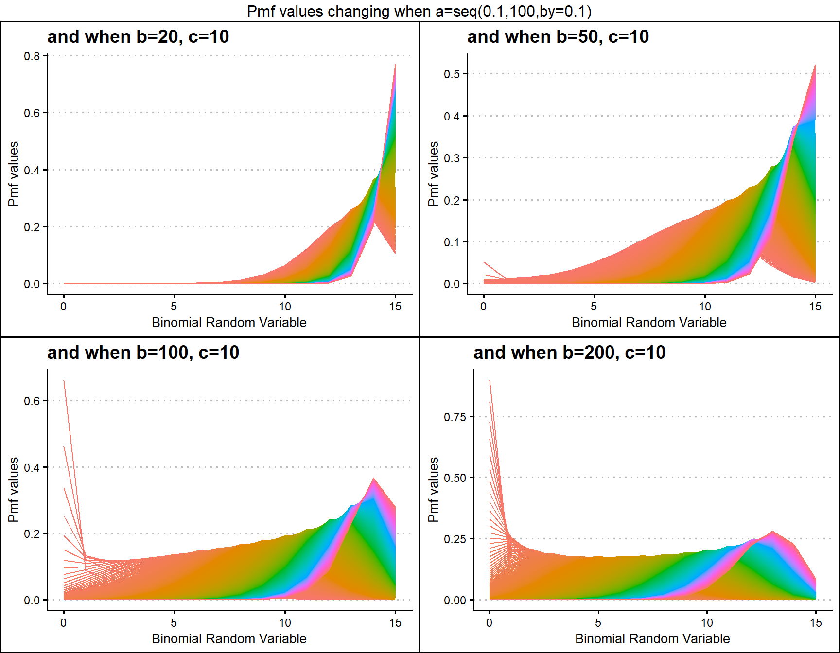

Probability Mass Function values for McDonald Generalized Beta-Binomial Distribution

McDonald Generalized Beta-Binomial Distribution is quite similar to GHGBB distribution only that it does not have any use of the Gaussian hyper-geometric function. Still it includes three shape parameters which are a,b and c. With necessary small twists in shape parameters it is possible to produce very vivid pmf values. Below are few plots explaining those scenarios.

a,b,c are in the domain region of above zero.

  b1c5 <- dMcGBBplot(a=seq(.5,10,by=.1),b=1,c=5,
                 plot_title="and when b=1, c=5",a_seq=T,b_seq=F)
b1.2c5 <- dMcGBBplot(a=seq(.5,10,by=.1),b=1.2,c=5,
                   plot_title="and when b=1.2, c=5",a_seq=T,b_seq=F)
  b3c5 <- dMcGBBplot(a=seq(.5,10,by=.1),b=3,c=5,
                 plot_title="and when b=3, c=5",a_seq=T,b_seq=F)
b3.2c5 <- dMcGBBplot(a=seq(.5,10,by=.1),b=3.2,c=5,
                   plot_title="and when b=3.2 c=5",a_seq=T,b_seq=F)

grid.arrange(b1c5,b1.2c5,b3c5,b3.2c5,nrow=2,
             top="Pmf values changing when a=seq(0.5,10,by=0.1)")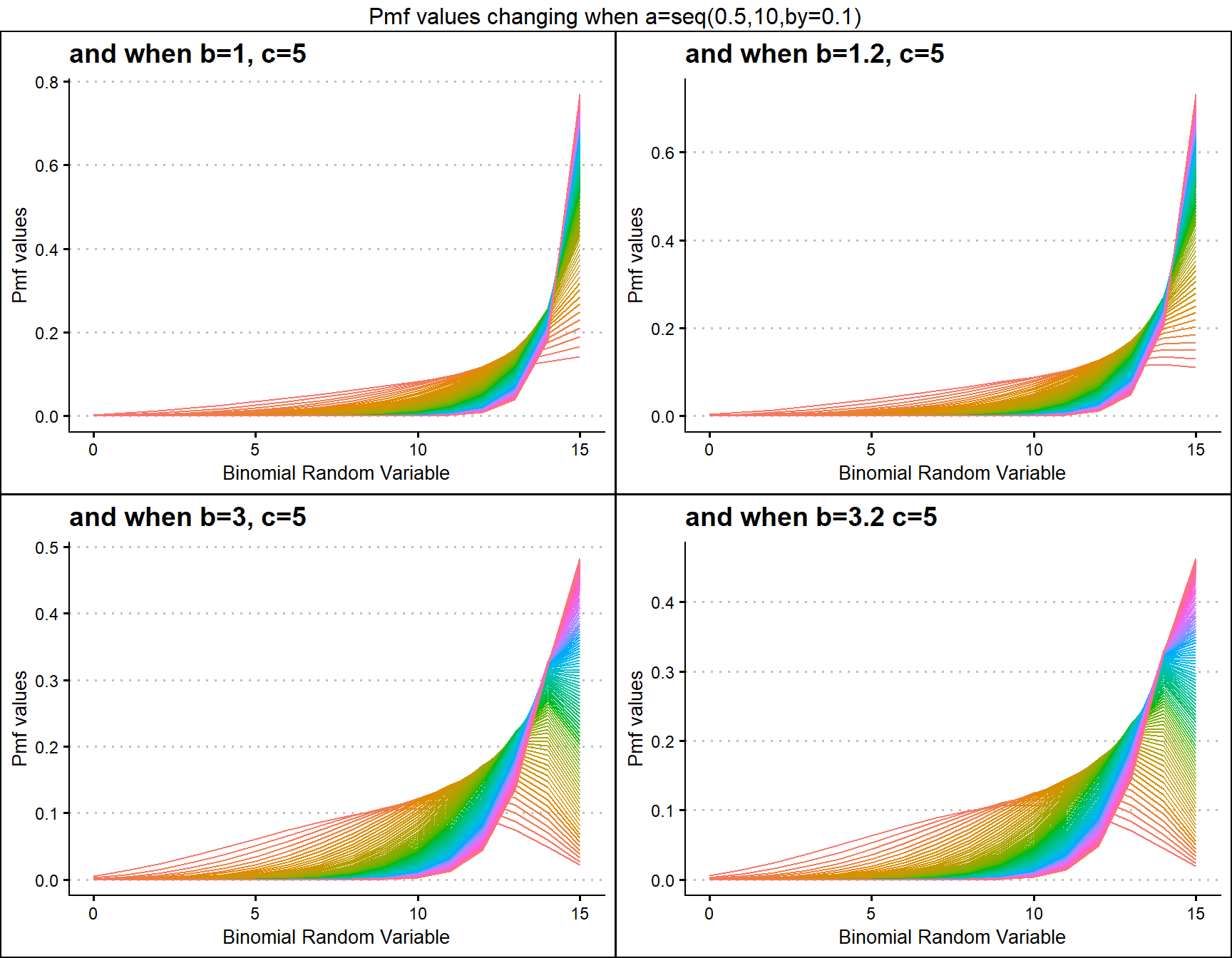

  b1c1 <- dMcGBBplot(a=seq(.5,100,by=.1),b=1,c=1,
                 plot_title="and when b=1, c=1",a_seq=T,b_seq=F)
b1c1.5 <- dMcGBBplot(a=seq(.5,100,by=.1),b=1,c=1.5,
                   plot_title="and when b=1, c=1.5",a_seq=T,b_seq=F)
  b1c2 <- dMcGBBplot(a=seq(.5,100,by=.1),b=1,c=2,
                 plot_title="and when b=1, c=2",a_seq=T,b_seq=F)
b1c2.5 <- dMcGBBplot(a=seq(.5,100,by=.1),b=1,c=2.5,
                   plot_title="and when b=1, c=2.5",a_seq=T,b_seq=F)

grid.arrange(b1c1,b1c1.5,b1c2,b1c2.5,nrow=2,
             top="Pmf values changing when a=seq(0.5,100,by=0.1)")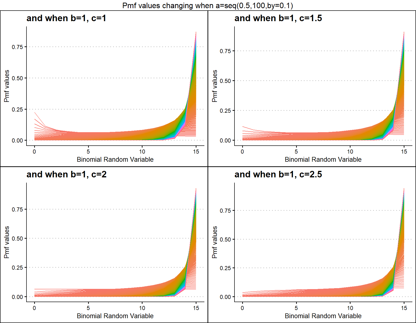

Probability Mass Function values for Gamma Binomial Distribution

Gamma Binomial Distribution has two shape parameters which influence the pmf values. They are namely a and b. These two parameters are inherited from the Gamma distribution when mixing it to the Binomial Distribution. Pmf values are plotted below according to a and b values change

a,b are in the domain region of above zero.

 b10 <- dGammaBinplot(a=seq(1,100,by=1),b=10,plot_title="and when b=10",a_seq= T)
 b50 <- dGammaBinplot(a=seq(1,100,by=1),b=50,plot_title="and when b=50",a_seq= T)
b100 <- dGammaBinplot(a=seq(1,100,by=1),b=100,plot_title="and when b=100",a_seq= T)
b200 <- dGammaBinplot(a=seq(1,100,by=1),b=200,plot_title="and when b=200",a_seq= T)

grid.arrange(b10,b50,b100,b200,nrow=2,top="Pmf values changing when a=seq(1,100,by=1)")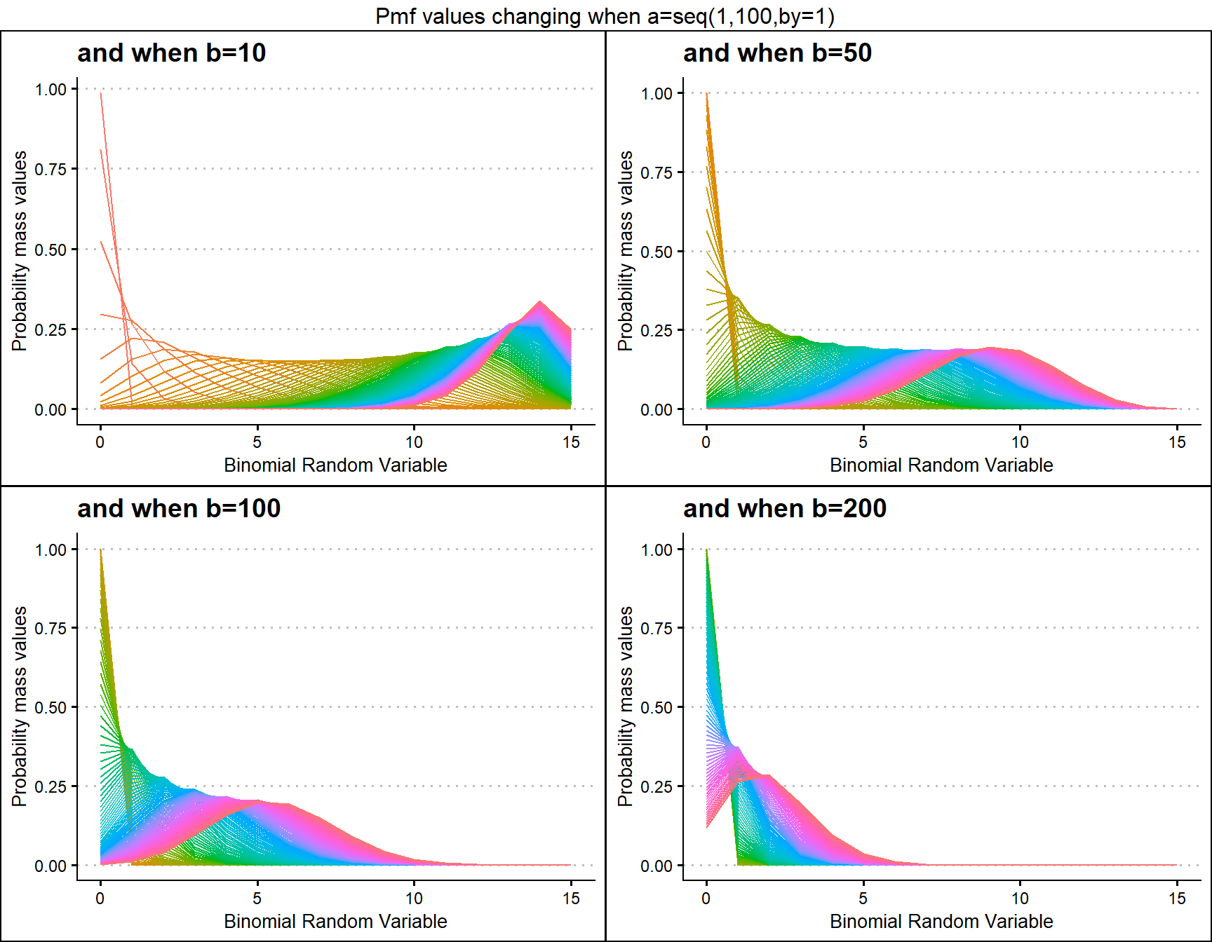

 a10 <- dGammaBinplot(b=seq(1,100,by=1),a=10,plot_title="and when a=10",a_seq= F)
 a50 <- dGammaBinplot(b=seq(1,100,by=1),a=50,plot_title="and when a=50",a_seq= F)
a100 <- dGammaBinplot(b=seq(1,100,by=1),a=100,plot_title="and when a=100",a_seq= F)
a200 <- dGammaBinplot(b=seq(1,100,by=1),a=200,plot_title="and when a=200",a_seq= F)

grid.arrange(a10,a50,a100,a200,nrow=2,top="Pmf values changing when b=seq(1,100,by=1)")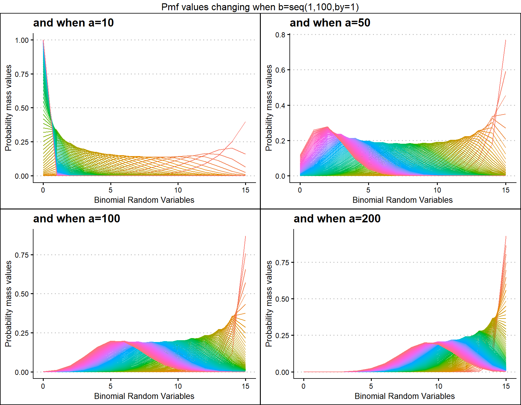

Probability Mass Function values for Grassia II Binomial Distribution

Grassia Binomial Distribution has two shape parameters which influence the pmf values. They are namely a and b. Pmf values are plotted below according to a and b values change

a,b are in the domain region of above zero.

 b1 <- dGrassiaIIBinplot(a=seq(0.1,10,by=0.1),b=0.1,plot_title="and when b=0.1",a_seq= T)
b25 <- dGrassiaIIBinplot(a=seq(0.1,10,by=0.1),b=0.25,plot_title="and when b=0.25",a_seq= T)
b35 <- dGrassiaIIBinplot(a=seq(0.1,10,by=0.1),b=0.35,plot_title="and when b=0.35",a_seq= T)
b40 <- dGrassiaIIBinplot(a=seq(0.1,10,by=0.1),b=0.4,plot_title="and when b=0.4",a_seq= T)

grid.arrange(b1,b25,b35,b40,nrow=2,top="Pmf values changing when a=seq(0.1,10,by=0.1)")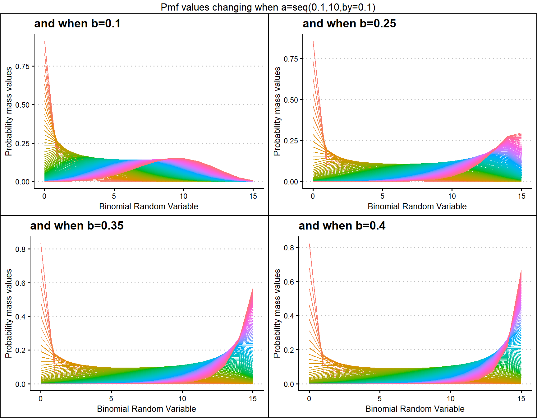

 a1 <- dGrassiaIIBinplot(b=seq(0.1,10,by=0.1),a=0.1,plot_title="and when a=0.1",a_seq= F)
a25 <- dGrassiaIIBinplot(b=seq(0.1,10,by=0.1),a=0.25,plot_title="and when a=0.25",a_seq= F)
 a5 <- dGrassiaIIBinplot(b=seq(0.1,10,by=0.1),a=0.5,plot_title="and when a=0.5",a_seq= F)
a10 <- dGrassiaIIBinplot(b=seq(0.1,10,by=0.1),a=1,plot_title="and when a=1",a_seq= F)

grid.arrange(a1,a25,a5,a10,nrow=2,top="Pmf values changing when b=seq(0.1,10,by=0.1)")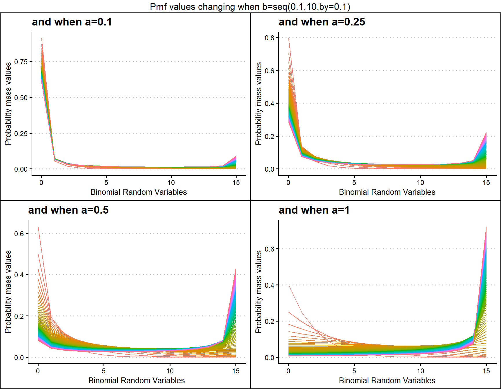

Alternate Binomial Distributions

Alternate Binomial Distributions were developed for the purpose of replacing Binomial Distribution. These distributions are similar to Binomial distribution but with special parameters which try to explain the over dispersion. Using pmf values it is possible to understand how much variation they can achieve as probability values generated. The functions which can develop pmf values for Alternate Binomial Distributions are

dAddBin - producing pmf values primarily for Additive Binomial Distribution.
dBetaCorrBin - producing pmf values primarily for Beta-Correlated Binomial Distribution.
dCOMPBin - producing pmf values primarily for COM Poisson Binomial Distribution.
dCorrBin - producing pmf values primarily for Correlated Binomial Distribution.
dMultiBin - producing pmf values primarily for Multiplicative Binomial Distribution.
dLMBin - producing pmf values primarily for Lovinson Multiplicative Binomial Distribution.

Specific functions were created for the purpose of making plot construction easy when there are more than two parameters involved. These functions are namely

dAddBinplot - plot function to Additive Binomial Distribution.
dBetaCorrBinplot - plot function to Beta Correlated Binomial Distribution.
dCOMPBinplot - plot function to COM Poisson Binomial Distribution.
dCorrBinplot - plot function to Correlated Binomial Distribution.
dMultiBinplot - plot function to Multiplicative Binomial Distribution.
dLMBinplot - producing pmf values primarily for Lovinson Multiplicative Binomial Distribution.

Probability Mass Function values for Additive Binomial Distribution

Additive Binomial distribution has one special parameter , which is the alpha value. Other than that it is included with a probability value. It is a replace for Binomial Distribution. Below is the plot generated to understand how its pmf values change.

p value in-between zero and one.
alpha value in-between negative one and positive one.

 alpha.005 <- dAddBinplot(p=seq(0.35,0.65,by=0.01),alpha=-0.005,
                       plot_title="and when alpha=-0.005",p_seq= T)
 alpha.001 <- dAddBinplot(p=seq(0.35,0.65,by=0.01),alpha=-0.001,
                       plot_title="and when alpha=-0.001",p_seq= T)
alpha0.001 <- dAddBinplot(p=seq(0.35,0.65,by=0.01),alpha=0.001,
                        plot_title="and when alpha=0.001",p_seq= T)
alpha0.005 <- dAddBinplot(p=seq(0.35,0.65,by=0.01),alpha=0.005,
                        plot_title="and when alpha=0.005",p_seq= T)

grid.arrange(alpha.005,alpha.001,alpha0.001,alpha0.005,nrow=2,
             top="Pmf values changing when p=seq(0.35,0.65,by=0.01)")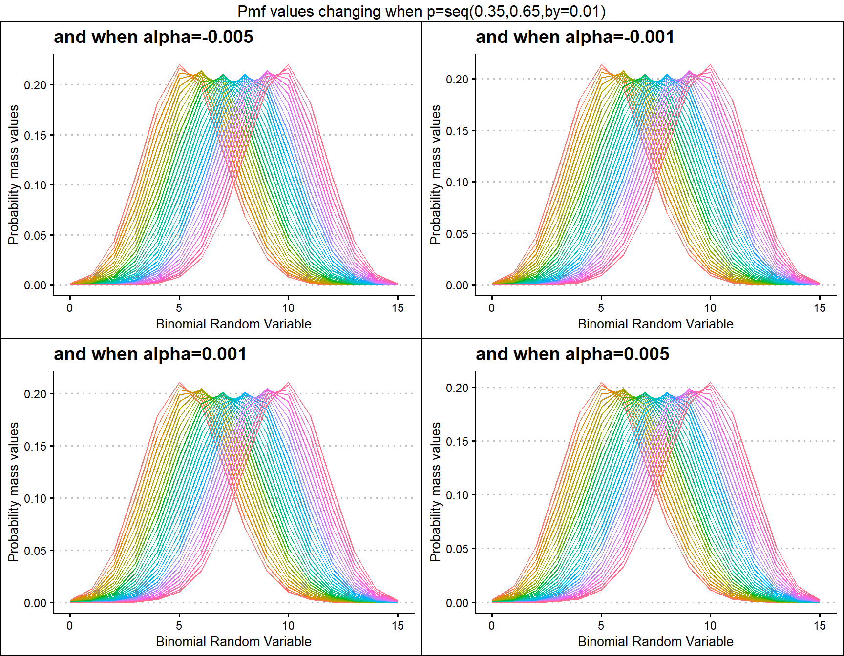

p.10 <- dAddBinplot(alpha=seq(.01,.1,by=0.001),p=0.1,
                  plot_title="and when p=0.10",p_seq= F)
p.30 <- dAddBinplot(alpha=seq(.01,.1,by=0.001),p=0.3,
                  plot_title="and when p=0.30",p_seq= F)
p.50 <- dAddBinplot(alpha=seq(.01,.1,by=0.001),p=0.5,
                  plot_title="and when p=0.50",p_seq= F)
p.85 <- dAddBinplot(alpha=seq(.01,.1,by=0.001),p=0.85,
                  plot_title="and when p=0.85",p_seq= F)

grid.arrange(p.10,p.30,p.50,p.85,nrow=2,
             top="Pmf values changing when alpha=seq(0.01,0.1,by=0.001)")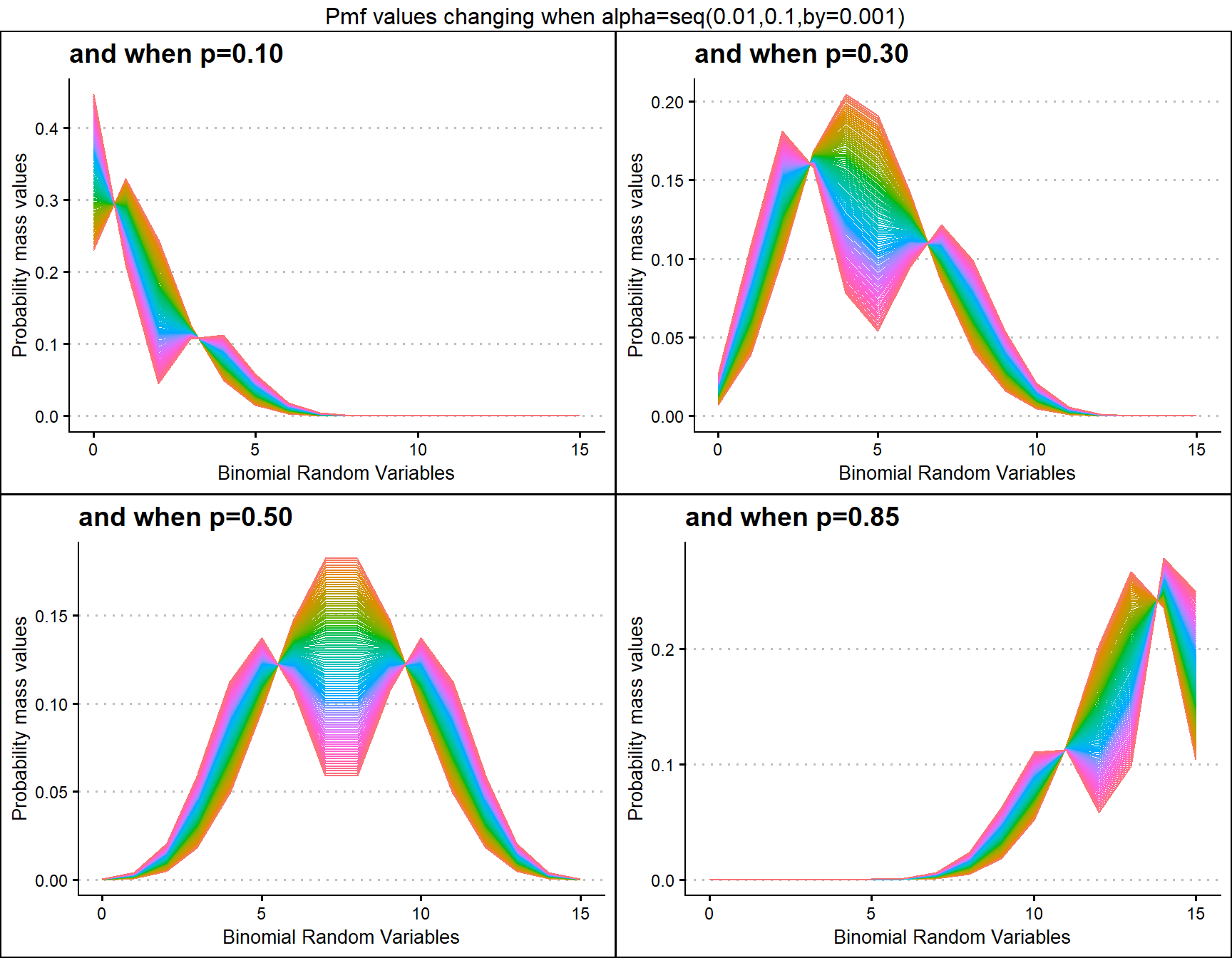

Probability Mass Function values for Beta-Correlated Binomial Distribution

Beta-Correlated Binomial distribution has three parameters in concern, where cov is the covariance from Correlated distribution and a,b are from the Beta Distribution. Mixing Binomial, Beta and Correlated distributions only we can develop the Beta-Correlated Binomial distribution. Below is the plot of explaining how their Pmf values change with respective to cov, a and b parameters.

cov is the covariance value in between negative infinity and positive infinity.
a, b are in the domain region of above zero.

 b16cov5 <- dBetaCorrBinplot(a=seq(10,100,by=0.1),b=16,cov=0.0005,
                 plot_title="and when b=16, cov=0.0005",a_seq=T,b_seq=F)
 b46cov5 <- dBetaCorrBinplot(a=seq(10,100,by=0.1),b=46,cov=0.0005,
                   plot_title="and when b=46, cov=0.0005",a_seq=T,b_seq=F)
 b76cov5 <- dBetaCorrBinplot(a=seq(10,100,by=0.1),b=76,cov=0.0005,
                 plot_title="and when b=76, cov=0.0005",a_seq=T,b_seq=F)
b106cov5 <- dBetaCorrBinplot(a=seq(10,100,by=0.1),b=106,cov=0.0005,
                   plot_title="and when b=106 cov=0.0005",a_seq=T,b_seq=F)

grid.arrange(b16cov5,b46cov5,b76cov5,b106cov5,nrow=2,
             top="Pmf values changing when a=seq(10,100,by=0.1)")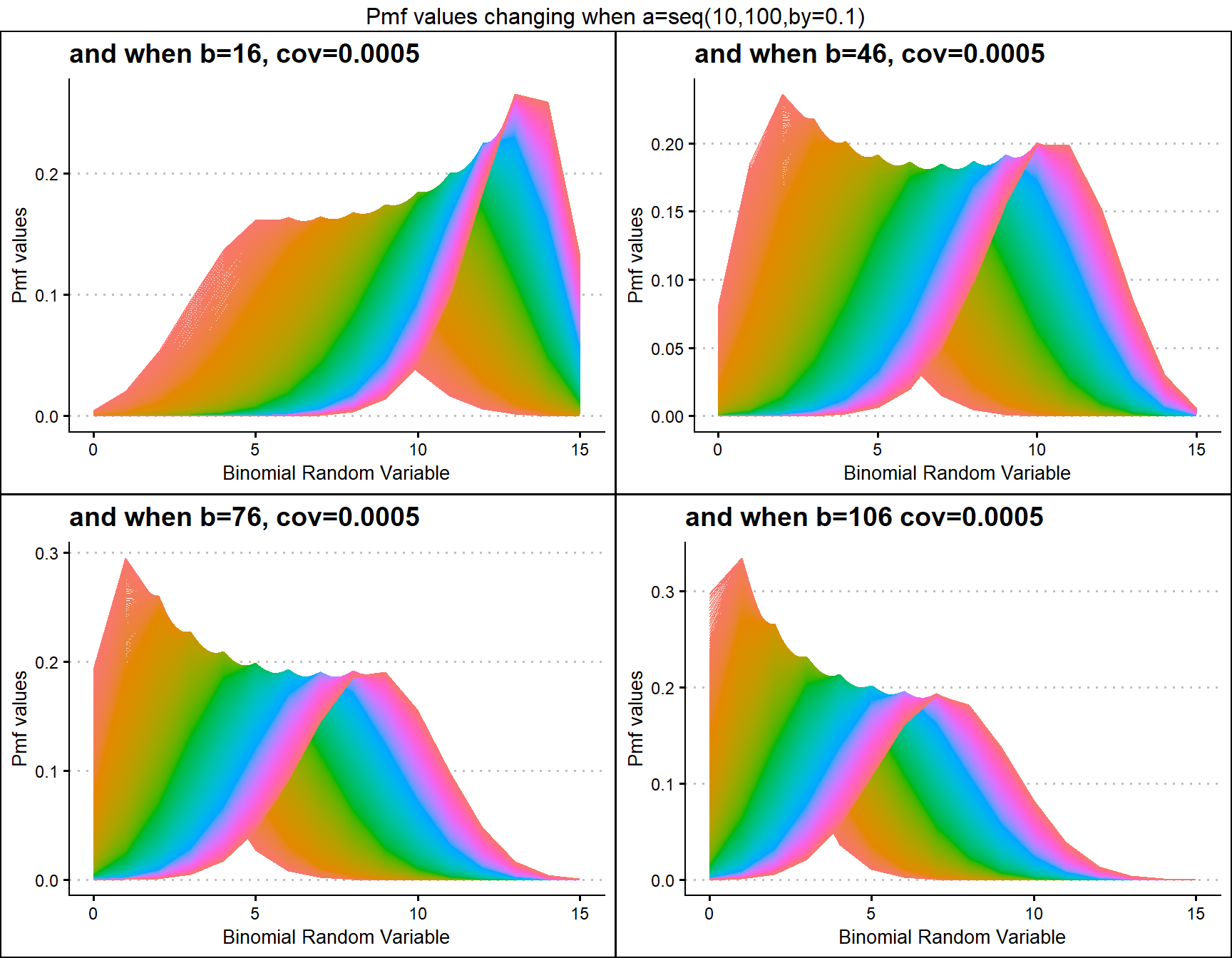

b10cov1 <- dBetaCorrBinplot(a=seq(15,100,by=0.1),b=10,cov=0.001,
                 plot_title="and when b=10, cov=0.001",a_seq=T,b_seq=F)
b10cov3 <- dBetaCorrBinplot(a=seq(15,100,by=0.1),b=10,cov=0.003,
                   plot_title="and when b=10, cov=0.003",a_seq=T,b_seq=F)
b10cov7 <- dBetaCorrBinplot(a=seq(15,100,by=0.1),b=10,cov=0.007,
                 plot_title="and when b=10, cov=0.007",a_seq=T,b_seq=F)
b10cov9 <- dBetaCorrBinplot(a=seq(15,100,by=0.1),b=10,cov=0.009,
                   plot_title="and when b=10, cov=0.009",a_seq=T,b_seq=F)

grid.arrange(b10cov1,b10cov3,b10cov7,b10cov9,nrow=2,
             top="Pmf values changing when a=seq(15,100,by=0.1)")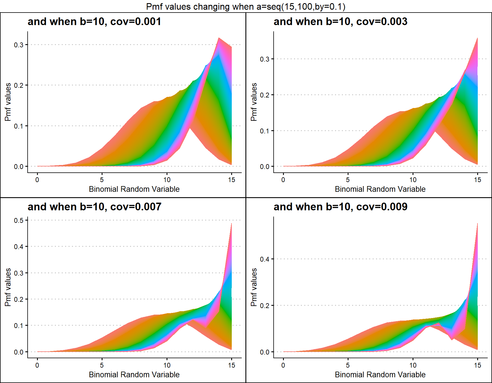

Probability Mass Function values for COM Poisson Binomial Distribution

COM Poisson Binomial distribution includes a probability value p and covariance value v. Which will be helpful in fitting over-dispersed Binomial Outcome data. Given below is the plot of how Pmf changes with relative to p and v.

p is the probability value in between zero and one.
v is the covariance value in between negative infinity and positive infinity.

 v.1 <- dCOMPBinplot(p=seq(0.25,0.75,by=0.001),v=-0.1,
                  plot_title="and when v=-0.1",p_seq= T)
v.01 <- dCOMPBinplot(p=seq(0.25,0.75,by=0.001),v=-0.01,
                   plot_title="and when v=-0.01",p_seq= T)
 v01 <- dCOMPBinplot(p=seq(0.25,0.75,by=0.001),v=1,
                  plot_title="and when v=1",p_seq= T)
 v05 <- dCOMPBinplot(p=seq(0.25,0.75,by=0.001),v=5,
                  plot_title="and when v=5",p_seq= T)

grid.arrange(v.1,v.01,v01,v05,nrow=2,
             top="Pmf values changing when p=seq(0.25,0.75,by=0.01)")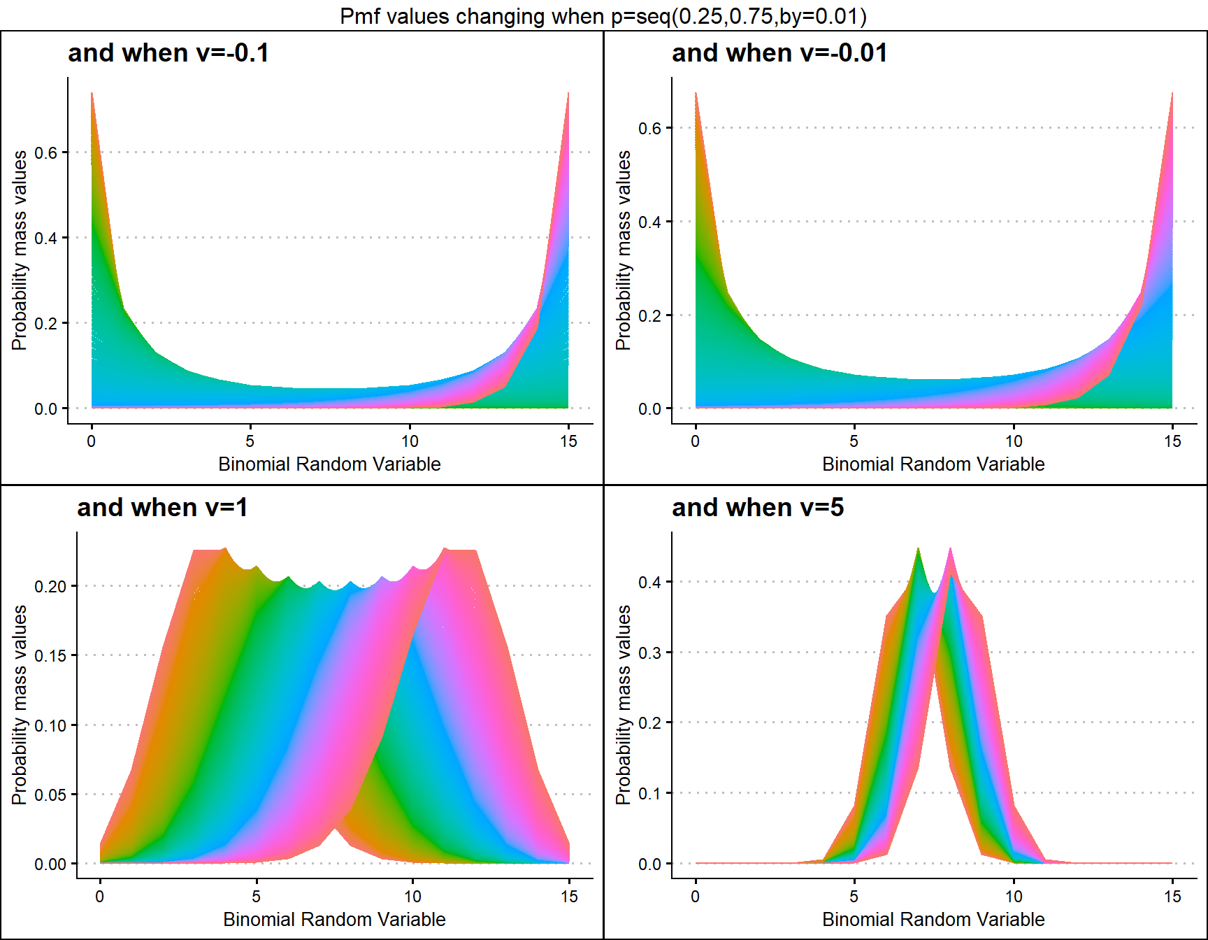

p0.25 <- dCOMPBinplot(v=seq(-0.5,0.5,by=.01),p=0.25,
                   plot_title="and when p=0.25",p_seq= F)
p0.45 <- dCOMPBinplot(v=seq(-0.5,0.5,by=.01),p=0.45,
                    plot_title="and when p=0.45",p_seq= F)
p0.50 <- dCOMPBinplot(v=seq(-0.5,0.5,by=.01),p=0.50,
                    plot_title="and when p=0.50",p_seq= F)
p0.65 <- dCOMPBinplot(v=seq(-0.5,0.5,by=.01),p=0.65,
                    plot_title="and when p=0.65",p_seq= F)

grid.arrange(p0.25,p0.45,p0.50,p0.65,nrow=2,
             top="Pmf values changing when v=seq(-0.5,0.5,by=0.01)")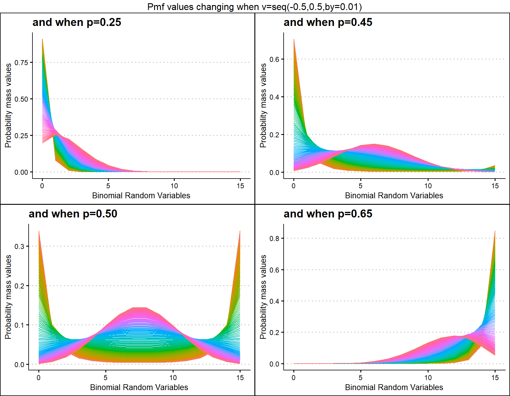

Probability Mass Function values for Correlated Binomial Distribution

Pmf values of Correlated Binomial distribution are influenced by covariance value cov and probability value p. They provide very nuance Pmf values when cov and p changes. Below given plot explains the situation of how Pmf values change with regarding to cov and p.

p is the probability value in between zero and one.
cov is the covariance value in between negative infinity and positive infinity.

cov.0001 <- dCorrBinplot(p=seq(0.35,0.75,by=0.001),cov=-0.0005,
                       plot_title="and when cov=-0.0005",p_seq= T)
cov.0005 <- dCorrBinplot(p=seq(0.35,0.75,by=0.001),cov=-0.0001,
                       plot_title="and when cov=-0.0001",p_seq= T)
 cov0.01 <- dCorrBinplot(p=seq(0.35,0.75,by=0.001),cov=0.01,
                        plot_title="and when cov=0.01",p_seq= T)
 cov0.05 <- dCorrBinplot(p=seq(0.35,0.75,by=0.001),cov=0.02,
                        plot_title="and when cov=0.02",p_seq= T)

grid.arrange(cov.0001,cov.0005,cov0.01,cov0.05,nrow=2,
             top="Pmf values changing when p=seq(0.35,0.75,by=0.001)")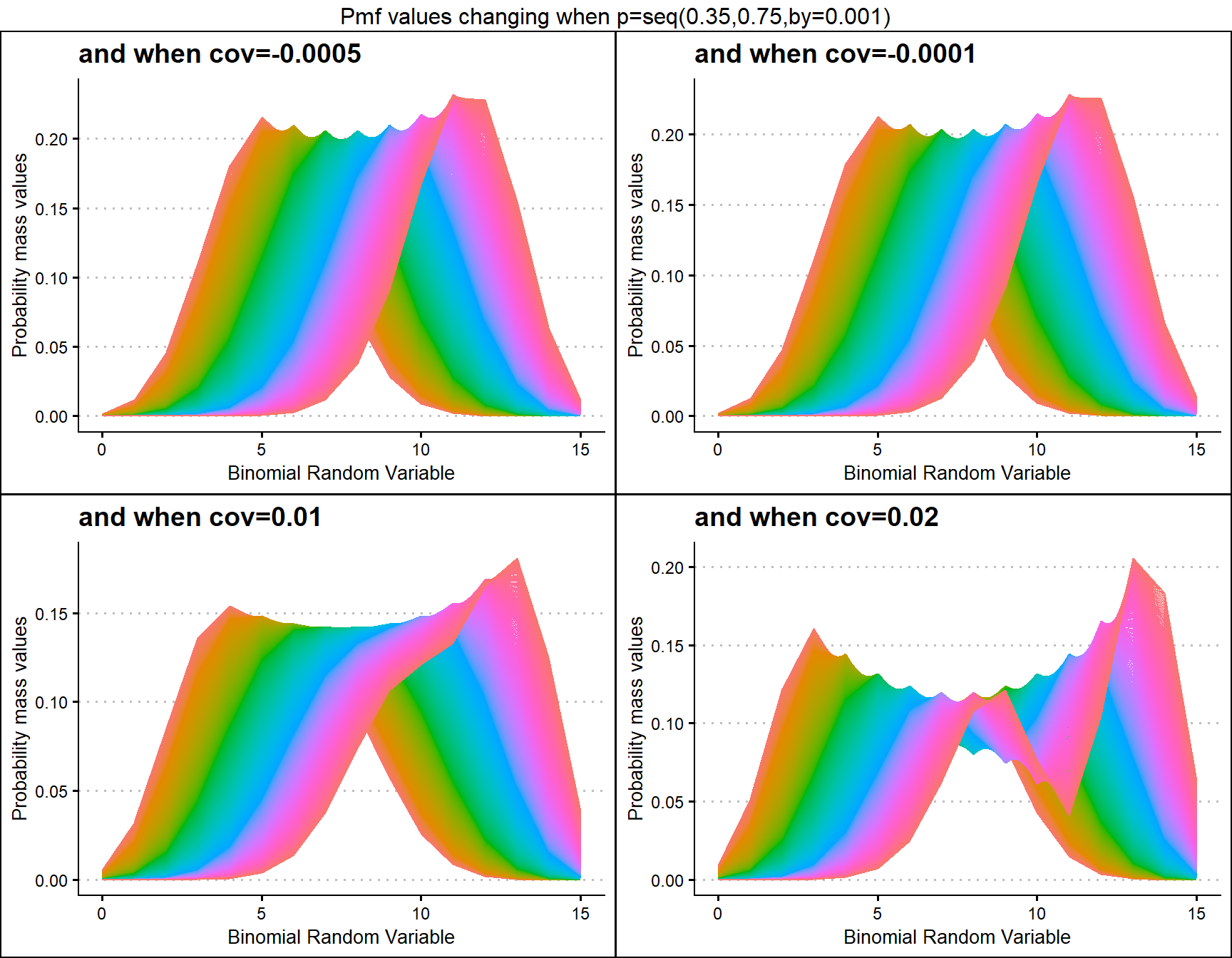

p0.075 <- dCorrBinplot(cov=seq(0.002,0.004,by=.0001),p=0.075,
                    plot_title="and when p=0.075",p_seq= F)
p0.175 <- dCorrBinplot(cov=seq(0.002,0.004,by=.0001),p=0.175,
                    plot_title="and when p=0.175",p_seq= F)
p0.275 <- dCorrBinplot(cov=seq(0.002,0.004,by=.0001),p=0.275,
                    plot_title="and when p=0.275",p_seq= F)
p0.375 <- dCorrBinplot(cov=seq(0.002,0.004,by=.0001),p=0.375,
                    plot_title="and when p=0.375",p_seq= F)

grid.arrange(p0.075,p0.175,p0.275,p0.375,nrow=2,
             top="Pmf values changing when cov=seq(0.002,0.004,by=0.0001)")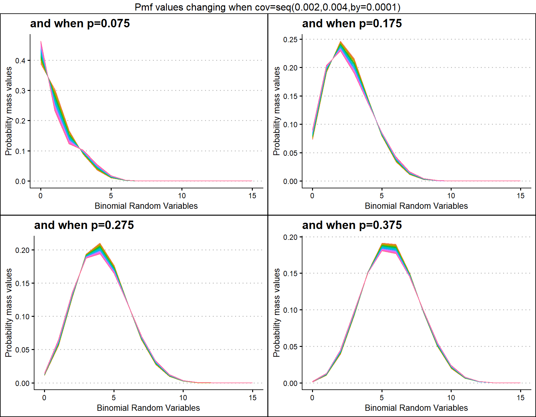

Probability Mass Function values for Multiplicative Binomial Distribution

Similar to COM Poisson Binomial and Correlated Binomial distributions this distribution is also influenced by the probability value. Although most influence can happen through the theta parameter as well. Therefore by changing values of theta parameter and p value we can clearly see how Pmf values change. Given below are the plots for that.

p is the probability value in between zero and one.
theta parameter is in the domain region of above zero.

 theta1 <- dMultiBinplot(p=seq(0.01,0.99,by=0.01),theta=1,
                       plot_title="and when theta=1",p_seq= T)
 theta5 <- dMultiBinplot(p=seq(0.01,0.99,by=0.01),theta=5,
                       plot_title="and when theta=5",p_seq= T)
theta10 <- dMultiBinplot(p=seq(0.01,0.99,by=0.01),theta=10,
                      plot_title="and when theta=10",p_seq= T)
theta50 <- dMultiBinplot(p=seq(0.01,0.99,by=0.01),theta=50,
                      plot_title="and when theta=50",p_seq= T)

grid.arrange(theta1,theta5,theta10,theta50,nrow=2,
             top="Pmf values changing when p=seq(0.01,0.99,by=0.01)")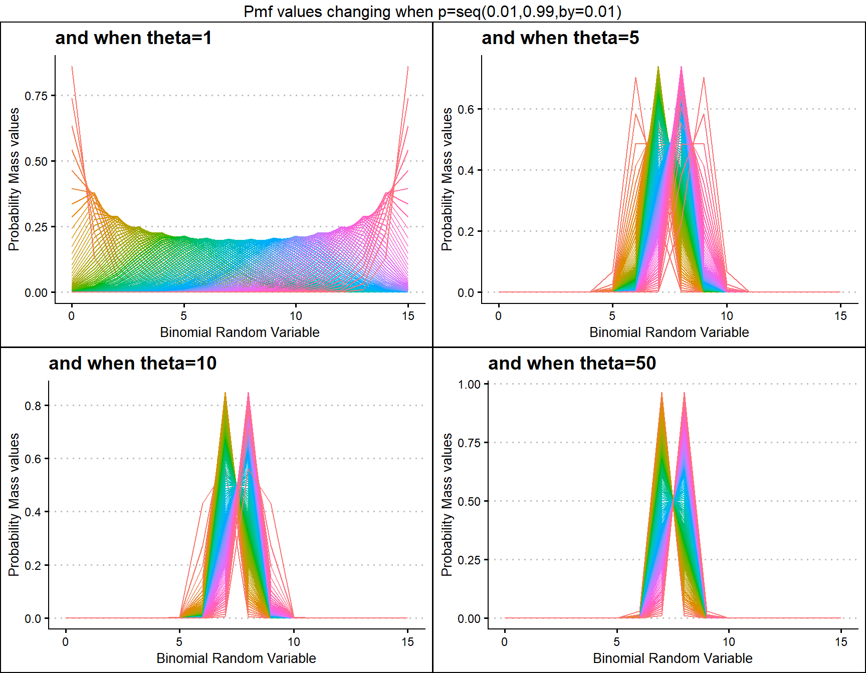

p0.10 <- dMultiBinplot(theta=seq(1,20,by=0.01),p=0.01,
                     plot_title="and when p=0.010",p_seq= F)
p0.25 <- dMultiBinplot(theta=seq(1,20,by=0.01),p=0.015,
                     plot_title="and when p=0.015",p_seq= F)
p0.50 <- dMultiBinplot(theta=seq(1,20,by=0.01),p=0.90,
                     plot_title="and when p=0.900",p_seq= F)
p0.75 <- dMultiBinplot(theta=seq(1,20,by=0.01),p=0.925,
                     plot_title="and when p=0.925",p_seq= F)

grid.arrange(p0.10,p0.25,p0.50,p0.75,nrow=2,
             top="Pmf values changing when theta=seq(1,20,by=0.01)")

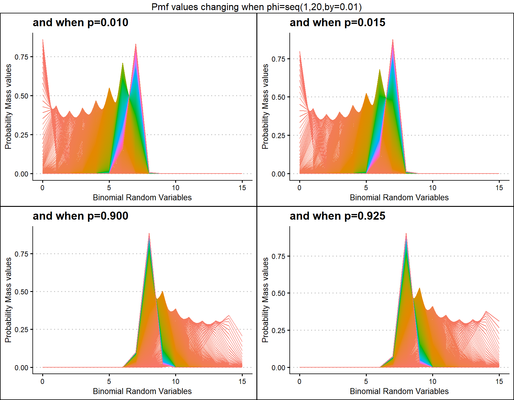
Probability Mass Function values for Lovinson Multiplicative Binomial Distribution

Similar to Multiplicative Binomial distribution. By changing values of phi parameter and p value we can clearly see how Pmf values change. Given below are the plots for that.

p is the probability value in between zero and one.
phi parameter is in the domain region of above zero.

 phi1 <- dLMBinplot(p=seq(0.01,0.99,by=0.01),phi=1,
                      plot_title="and when phi=1",p_seq= T)
 phi5 <- dLMBinplot(p=seq(0.01,0.99,by=0.01),phi=5,
                      plot_title="and when phi=5",p_seq= T)
phi10 <- dLMBinplot(p=seq(0.01,0.99,by=0.01),phi=10,
                       plot_title="and when phi=10",p_seq= T)
phi50 <- dLMBinplot(p=seq(0.01,0.99,by=0.01),phi=50,
                       plot_title="and when phi=50",p_seq= T)

grid.arrange(phi1,phi5,phi10,phi50,nrow=2,
             top="Pmf values changing when p=seq(0.01,0.99,by=0.01)")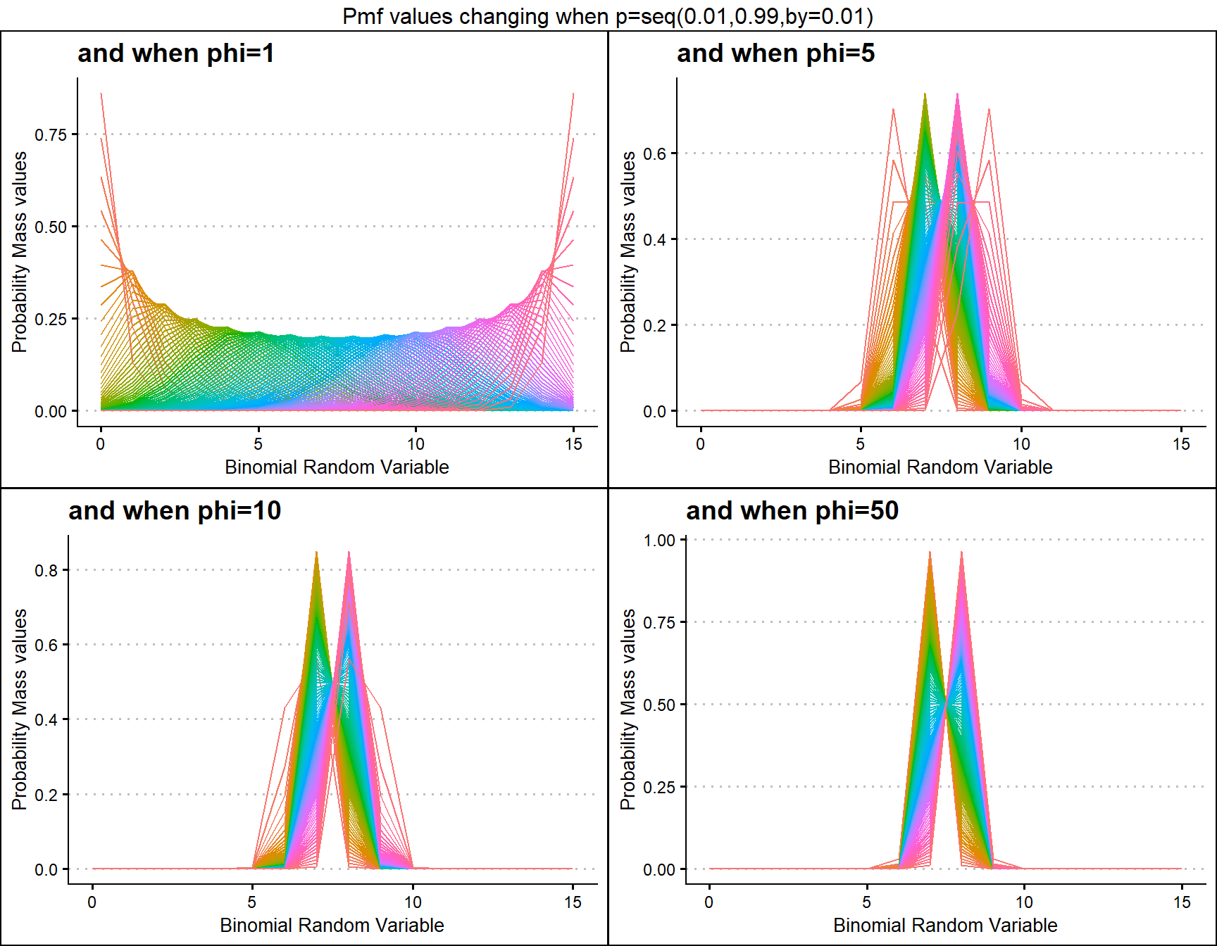

p0.10 <- dLMBinplot(phi=seq(1,20,by=0.01),p=0.01,
                     plot_title="and when p=0.010",p_seq= F)
p0.25 <- dLMBinplot(phi=seq(1,20,by=0.01),p=0.015,
                     plot_title="and when p=0.015",p_seq= F)
p0.50 <- dLMBinplot(phi=seq(1,20,by=0.01),p=0.90,
                     plot_title="and when p=0.900",p_seq= F)
p0.75 <- dLMBinplot(phi=seq(1,20,by=0.01),p=0.925,
                     plot_title="and when p=0.925",p_seq= F)

grid.arrange(p0.10,p0.25,p0.50,p0.75,nrow=2,
             top="Pmf values changing when phi=seq(1,20,by=0.01)")

Binomial Mixture and Alternate Binomial Distributions PMF values