Pdf values of Unit Bounded Distributions or Mixing Distributions
Source:vignettes/Mixing_Distributions_dxxx.Rmd
Mixing_Distributions_dxxx.RmdIT WOULD BE CLEARLY BENEFICIAL FOR YOU BY USING THE RMD FILES IN THE GITHUB DIRECTORY FOR FURTHER EXPLANATION OR UNDERSTANDING OF THE R CODE FOR THE RESULTS OBTAINED IN THE VIGNETTES.
Each distribution is unique when it comes to producing Probability density values. Therefore in order to understand how they react the Pdf values have been plotted below. There are distributions starting with no shape parameters to three shape parameters. Which would be useful in modelling data. The functions which provide the Pdf values are
-
dUNI- Producing Pdf values primarily for Uniform Distribution. -
dTRI- Producing Pdf values primarily for Triangular Distribution. -
dBETA- Producing Pdf values primarily for Beta Distribution. -
dKUM- Producing Pdf values primarily for Kumaraswamy Distribution. -
dGHGBeta- Producing Pdf values primarily for Gaussian Hyper-geometric Generalized Beta Distribution. -
dGBeta1- Producing Pdf values primarily for Generalized Beta Type 1 Distribution. -
dGAMMA- Producing Pdf values primarily for Gamma Distribution.
With the increase of shape parameters which influence the Pdf values new functions have be developed to plot these pdf values against probability values. These plot functions are specifically for distributions with more than one parameter. These plot are named below as
-
dBETAplot- Function to plot Pdf values for Beta Distribution. -
dKUMplot- Function to plot Pdf values for Kumaraswamy Distribution. -
dGHGBetaplot- Function to plot Pdf values for Gaussian Hyper-geometric Generalized Beta Distribution. -
dGBeta1plot- Function to plot Pdf values for Generalized Beta Type 1 Distribution. -
dGAMMAplot- Function to plot Pdf values for Gamma Distribution.
It should be noted that better techniques should be found to express pdf values changing with respective to all shape parameters changing simultaneously. Distributions with two or more parameters will be restricted as 3D plotting is not enough to the task at hand.
Probability Density values for Uniform Distribution
Uniform distribution does not involve any shape parameter and no parameter at all. Therefore no significant fluctuation in Pdf values. Yet plotted below
prob <- seq(0.01,0.99,by=0.01)
pdfv <- dUNI(prob)$pdf
data <- data.frame(prob,pdfv)
ggplot(data)+
  geom_line(aes(x=data$prob,y=data$pdfv))+
  xlab("Vector of Probabilities")+
  ylab("Probability density values")+
  ggthemes::theme_clean()+
  ggtitle("Pdf values changing")
Probability Density values for Triangular Distribution
Triangular distribution includes only one parameter, which is the mode value in-between zero and one. Below is the plot explaining how pdf values change when mode changes
prob <- seq(0.01,0.99,by=0.01)
mode <- seq(0.01,0.99,by=0.01)
output <- matrix(ncol =length(mode) ,nrow=length(prob))
for (i in 1:length(mode))
  {
   output[,i]<-dTRI(prob,mode[i])$pdf
  }
data <- data.frame(prob,output)
data <- melt(data,id.vars ="prob" )
ggplot(data,aes(prob,value,col=variable))+
  geom_line()+guides(fill=FALSE,color=FALSE)+
  xlab("Vector of Probabilities")+
  ylab("Probability density values")+ggthemes::theme_clean()+
  ggtitle("Pdf values changing when c=seq(0.01,0.09,by0.01)")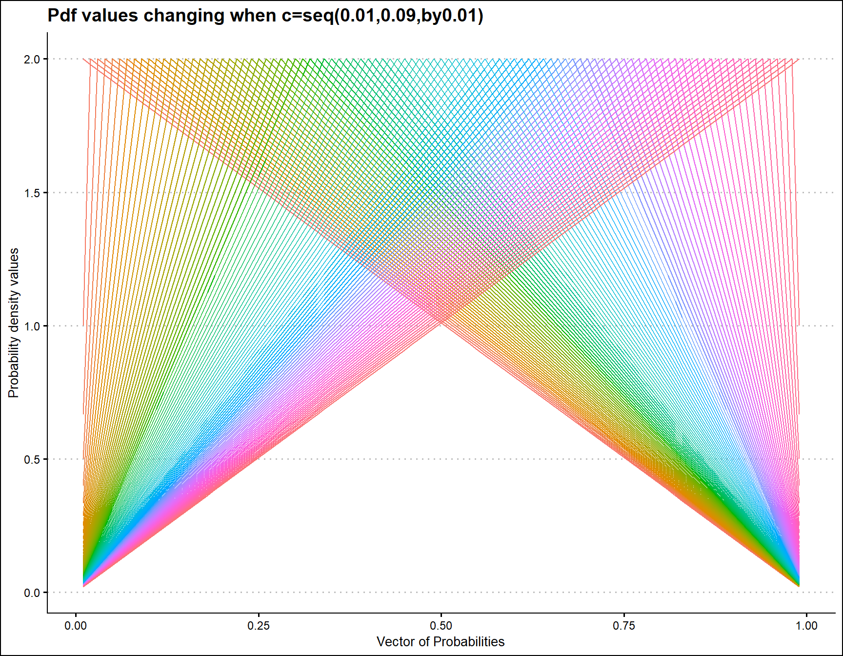
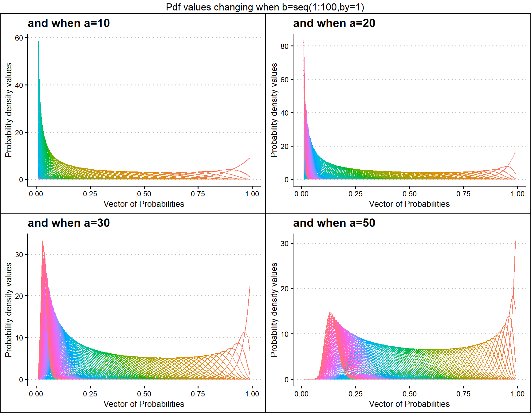
Probability Density values for Beta Distribution
Beta Distribution has two shape parameters, which are a and b. They give the opportunity to acquire variety of pdf values for any each combination of a and b. Below is the brief explanation of how it occurs.
- a,b are in the domain region of above zero.
 b10 <- dBETAplot(a=seq(1,100,by=1),b=10,plot_title="and when b=10",a_seq= T)
 b50 <- dBETAplot(a=seq(1,100,by=1),b=50,plot_title="and when b=50",a_seq= T)
b100 <- dBETAplot(a=seq(1,100,by=1),b=100,plot_title="and when b=100",a_seq= T)
b200 <- dBETAplot(a=seq(1,100,by=1),b=200,plot_title="and when b=200",a_seq= T)

grid.arrange(b10,b50,b100,b200,nrow=2,top="Pdf values changing when a=seq(1:100,by=1)")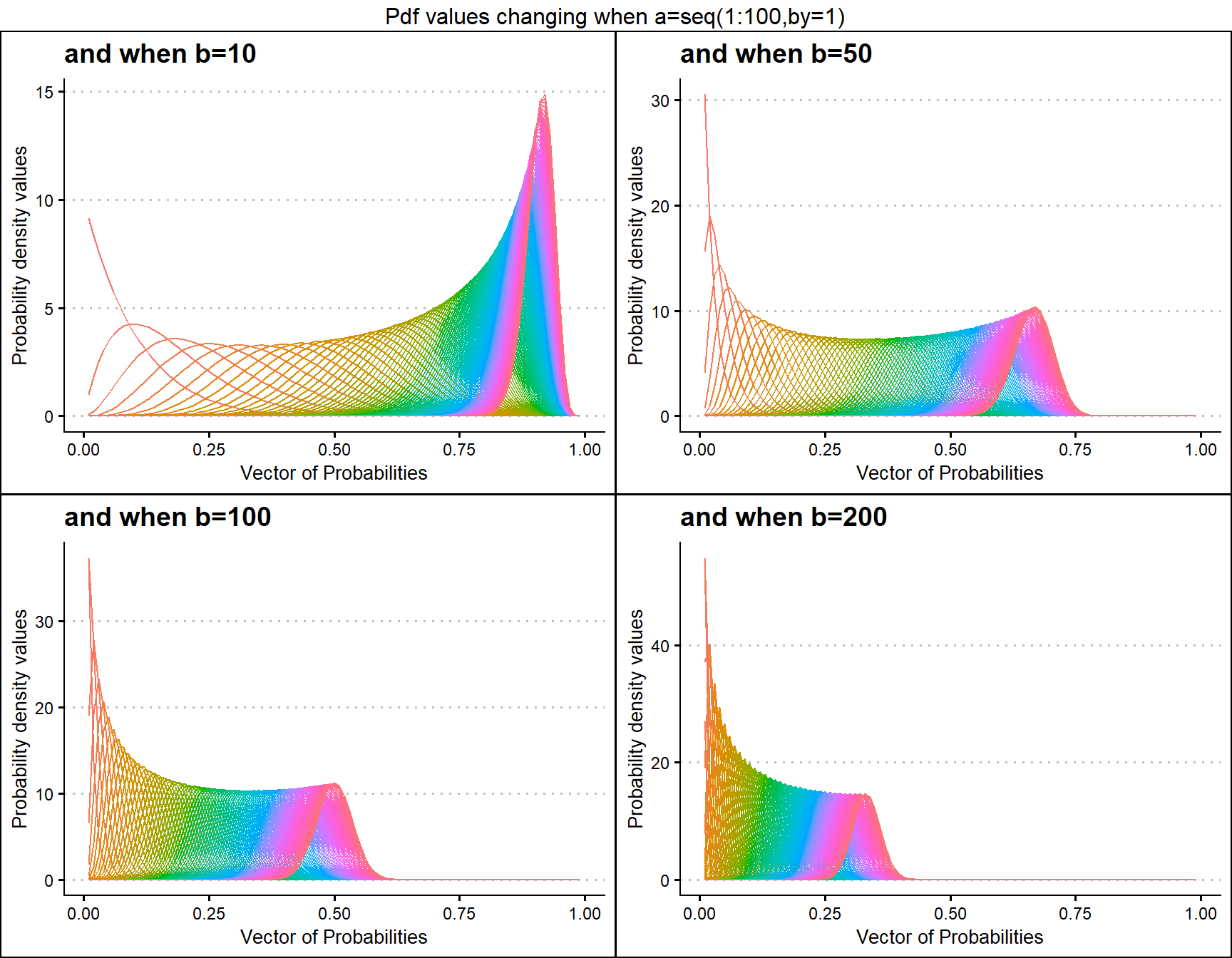
 a10 <- dBETAplot(b=seq(1,100,by=1),a=10,plot_title="and when a=10",a_seq= F)
 a50 <- dBETAplot(b=seq(1,100,by=1),a=50,plot_title="and when a=50",a_seq= F)
a100 <- dBETAplot(b=seq(1,100,by=1),a=100,plot_title="and when a=100",a_seq= F)
a200 <- dBETAplot(b=seq(1,100,by=1),a=200,plot_title="and when a=200",a_seq= F)

grid.arrange(a10,a50,a100,a200,nrow=2,top="Pdf values changing when b=seq(1:100,by=1)")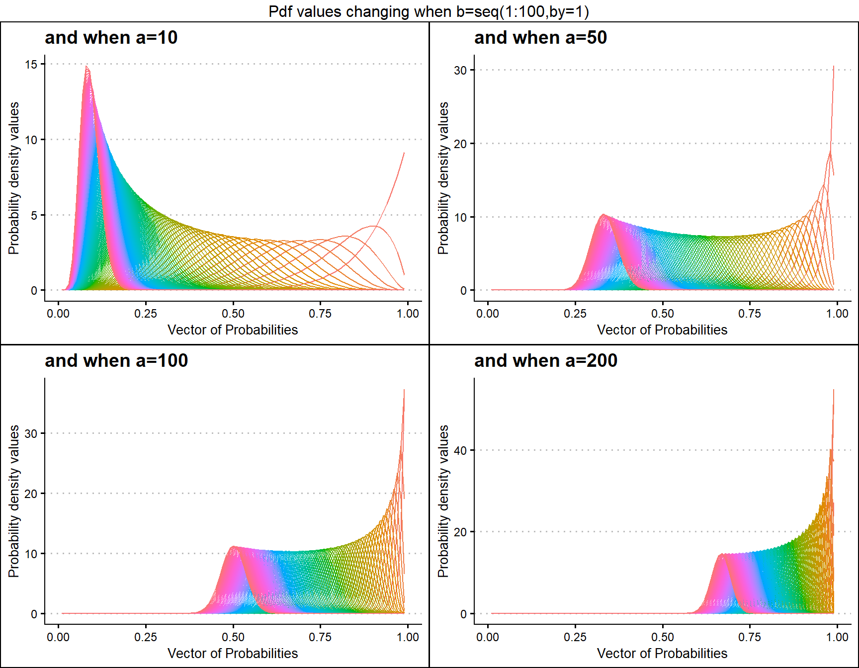
Probability Density values for Kumaraswamy Distribution
Two shape parameters are included in Kumaraswamy distribution, similar to Beta distribution. Yet, it is widely believed that this distribution covers the pdf value variations which Beta distribution cannot produce. Below are plots to understand how shape parameters affect pdf values.
- a,b are in the domain region of above zero.
 b10 <- dKUMplot(a=seq(1,100,by=1),b=10,plot_title="and when b=10",a_seq=T)
 b50 <- dKUMplot(a=seq(1,100,by=1),b=50,plot_title="and when b=50",a_seq=T)
b100 <- dKUMplot(a=seq(1,100,by=1),b=100,plot_title="and when b=100",a_seq=T)
b200 <- dKUMplot(a=seq(1,100,by=1),b=200,plot_title="and when b=200",a_seq=T)

grid.arrange(b10,b50,b100,b200,nrow=2,top="Pdf values changing when a=seq(1:100,by=1)")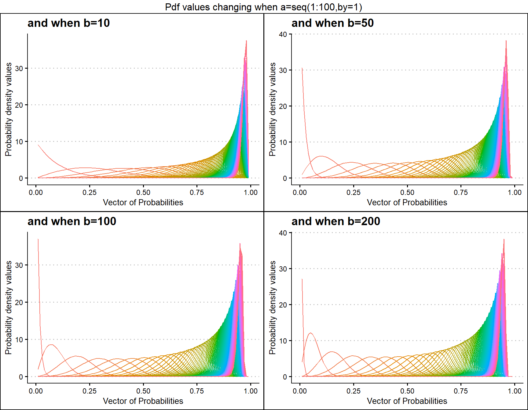
 a3 <- dKUMplot(b=seq(1,100,by=1),a=3,plot_title="and when a=3",a_seq=F)
 a5 <- dKUMplot(b=seq(1,100,by=1),a=5,plot_title="and when a=5",a_seq=F)
a10 <- dKUMplot(b=seq(1,100,by=1),a=10,plot_title="and when a=10",a_seq=F)
a15 <- dKUMplot(b=seq(1,100,by=1),a=15,plot_title="and when a=15",a_seq=F)

grid.arrange(a3,a5,a10,a15,nrow=2,top="Pdf values changing when b=seq(1:100,by=1)")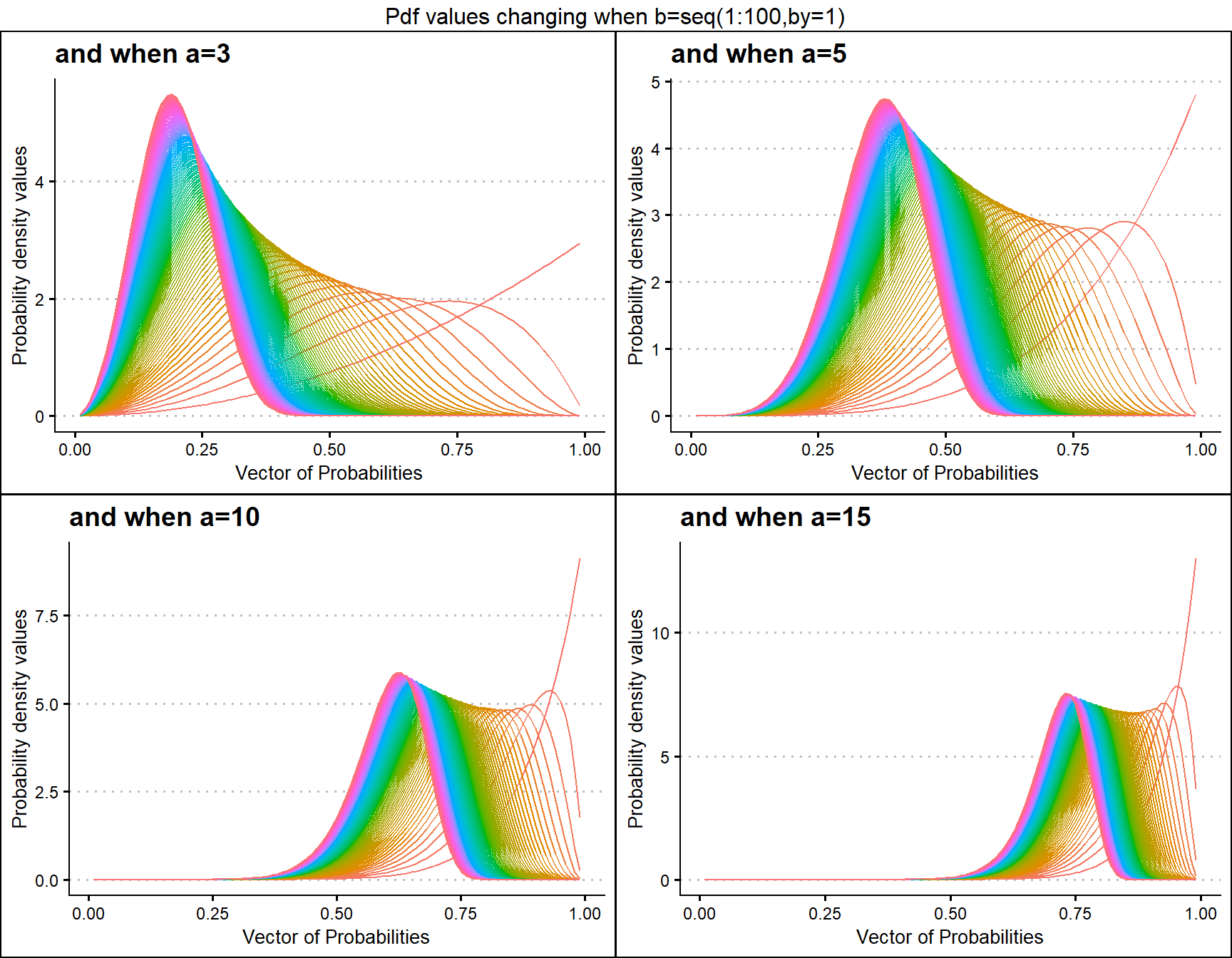
Probability Density values for Gaussian Hyper-geometric Generalized Beta Distribution
This distribution is completely different from others, as it contains a binomial trial value n. n occurs because it was reverse engineered using Gaussian Hyper-geometric Generalized Beta Binomial distribution. This has three shape parameters that are a,b and c. Below are the plots describing how pdf values change with respective to shape parameters.
- a,b,c are in the domain region of above zero.
- n is a natural number which should only take values of 0,1,2,… .
 b10c.5 <- dGHGBetaplot(n=10,a=seq(.1,100,by=.1),b=10,c=.5,
                     plot_title="and when b=10, c=0.5",a_seq=T,b_seq=F)
 b50c.5 <- dGHGBetaplot(n=10,a=seq(.1,100,by=.1),b=50,c=.5,
                     plot_title="and when b=50, c=0.5",a_seq=T,b_seq=F)
b100c.5 <- dGHGBetaplot(n=10,a=seq(.1,100,by=.1),b=100,c=.5,
                      plot_title="and when b=100, c=0.5",a_seq=T,b_seq=F)
b200c.5 <- dGHGBetaplot(n=10,a=seq(.1,100,by=.1),b=130,c=.5,
                      plot_title="and when b=130, c=0.5",a_seq=T,b_seq=F)

grid.arrange(b10c.5,b50c.5,b100c.5,b200c.5,nrow=2,
             top="Pdf values changing when a=seq(0.1,100,by=0.1)")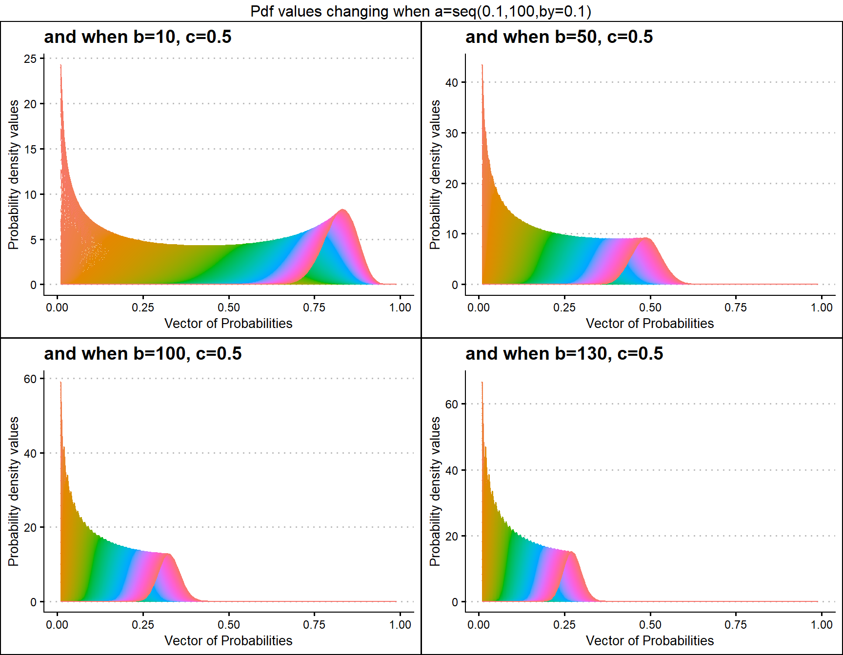
 b10c1 <- dGHGBetaplot(n=10,a=seq(.1,100,by=.1),b=10,c=1,
                    plot_title="and when b=10, c=1",a_seq=T,b_seq=F)
 b50c1 <- dGHGBetaplot(n=10,a=seq(.1,100,by=.1),b=50,c=1,
                    plot_title="and when b=50, c=1",a_seq=T,b_seq=F)
b100c1 <- dGHGBetaplot(n=10,a=seq(.1,100,by=.1),b=100,c=1,
                     plot_title="and when b=100, c=1",a_seq=T,b_seq=F)
b200c1 <- dGHGBetaplot(n=10,a=seq(.1,100,by=.1),b=130,c=1,
                     plot_title="and when b=200, c=1",a_seq=T,b_seq=F)

grid.arrange(b10c1,b50c1,b100c1,b200c1,nrow=2,
             top="Pdf values changing when a=seq(0.1,100,by=0.1)")
 b10c5 <- dGHGBetaplot(n=10,a=seq(.1,100,by=.1),b=10,c=5,
                    plot_title="and when b=10, c=5",a_seq=T,b_seq=F)
 b50c5 <- dGHGBetaplot(n=10,a=seq(.1,100,by=.1),b=50,c=5,
                    plot_title="and when b=50, c=5",a_seq=T,b_seq=F)
b100c5 <- dGHGBetaplot(n=10,a=seq(.1,100,by=.1),b=100,c=5,
                     plot_title="and when b=100, c=5",a_seq=T,b_seq=F)
b200c5 <- dGHGBetaplot(n=10,a=seq(.1,100,by=.1),b=150,c=5,
                     plot_title="and when b=150, c=5",a_seq=T,b_seq=F)

grid.arrange(b10c5,b50c5,b100c5,b200c5,nrow=2,
             top="Pdf values changing when a=a=seq(0.1,100,by=0.1)")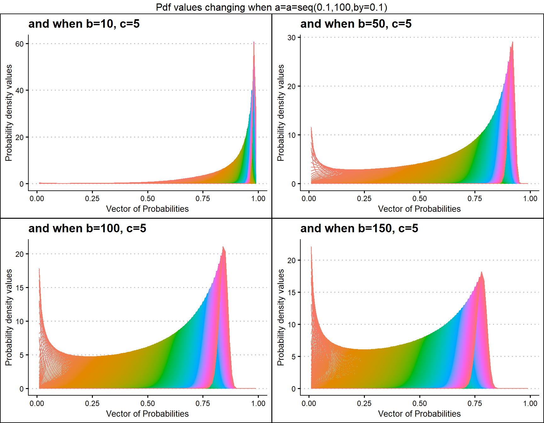
 b10c10 <- dGHGBetaplot(n=10,a=seq(.1,100,by=.1),b=10,c=10,
                     plot_title="and when b=10, c=10",a_seq=T,b_seq=F)
 b50c10 <- dGHGBetaplot(n=10,a=seq(.1,100,by=.1),b=50,c=10,
                     plot_title="and when b=50, c=10",a_seq=T,b_seq=F)
b100c10 <- dGHGBetaplot(n=10,a=seq(.1,100,by=.1),b=100,c=10,
                      plot_title="and when b=100, c=10",a_seq=T,b_seq=F)
b200c10 <- dGHGBetaplot(n=10,a=seq(.1,100,by=.1),b=200,c=10,
                      plot_title="and when b=200, c=10",a_seq=T,b_seq=F)

grid.arrange(b10c10,b50c10,b100c10,b200c10,nrow=2,
             top="Pdf values changing when a=seq(0.1,100,by=0.1)")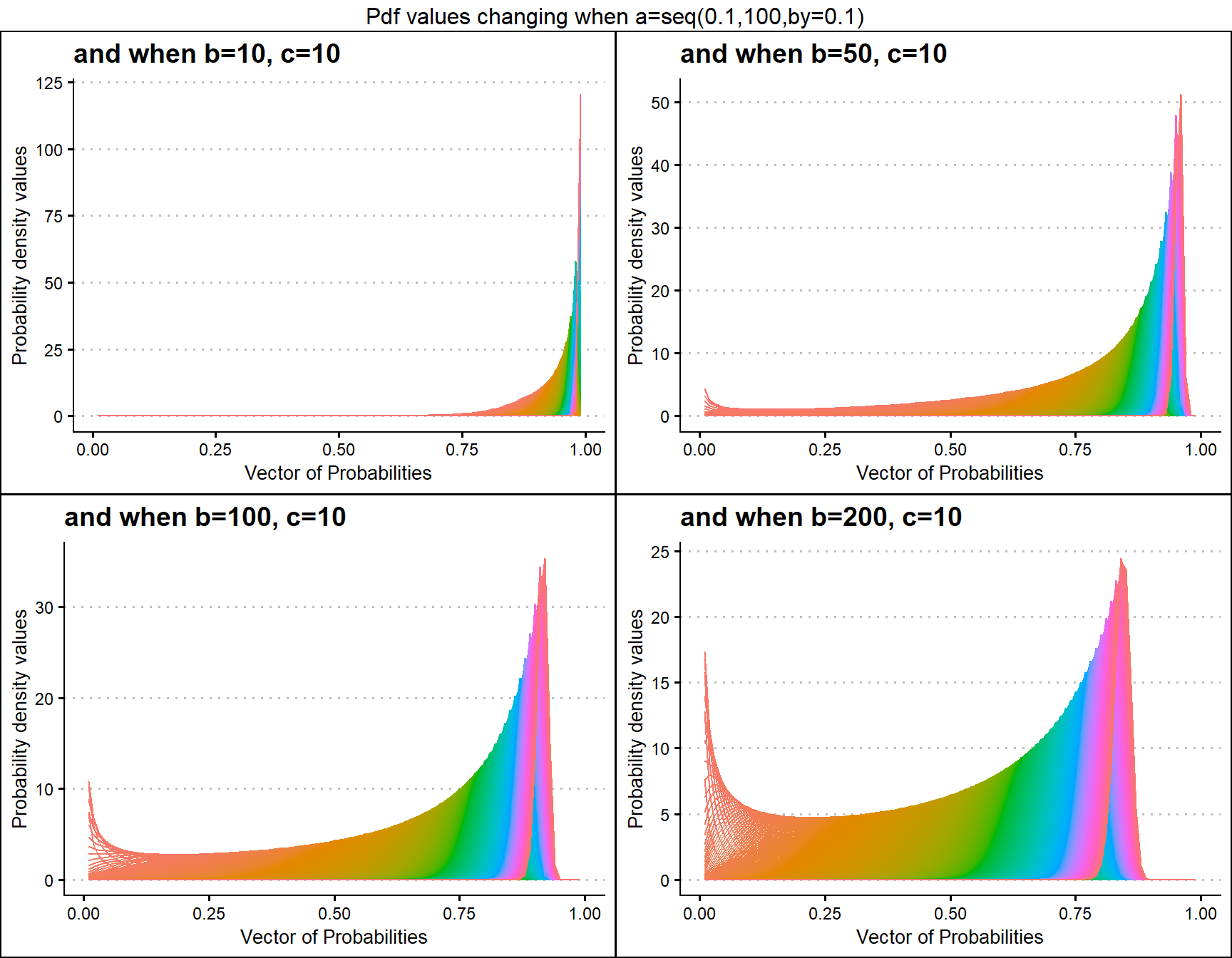
Probability Density values for Generalized Beta Type1 Distribution
Generalized Beta Type 1 distribution has three shape parameters that are a,b and c. With proper values for a,b,c they can behave similarly to Beta or Kumaraswamy Distribution. Plots have been generated where with a,b,c values change and pdf values too.
- a,b,c are in the domain region of above zero.
 b10c.5 <- dGBeta1plot(a=seq(.1,100,by=.1),b=10,c=.5,
                    plot_title="and when b=10, c=0.5",a_seq=T,b_seq=F)
 b50c.5 <- dGBeta1plot(a=seq(.1,100,by=.1),b=50,c=.5,
                    plot_title="and when b=50, c=0.5",a_seq=T,b_seq=F)
b100c.5 <- dGBeta1plot(a=seq(.1,100,by=.1),b=100,c=.5,
                     plot_title="and when b=100, c=0.5",a_seq=T,b_seq=F)
b130c.5 <- dGBeta1plot(a=seq(.1,100,by=.1),b=130,c=.5,
                     plot_title="and when b=130, c=0.5",a_seq=T,b_seq=F)

grid.arrange(b10c.5,b50c.5,b100c.5,b130c.5,nrow=2,
             top="Pdf values changing when a=seq(0.1,100,by=0.1)")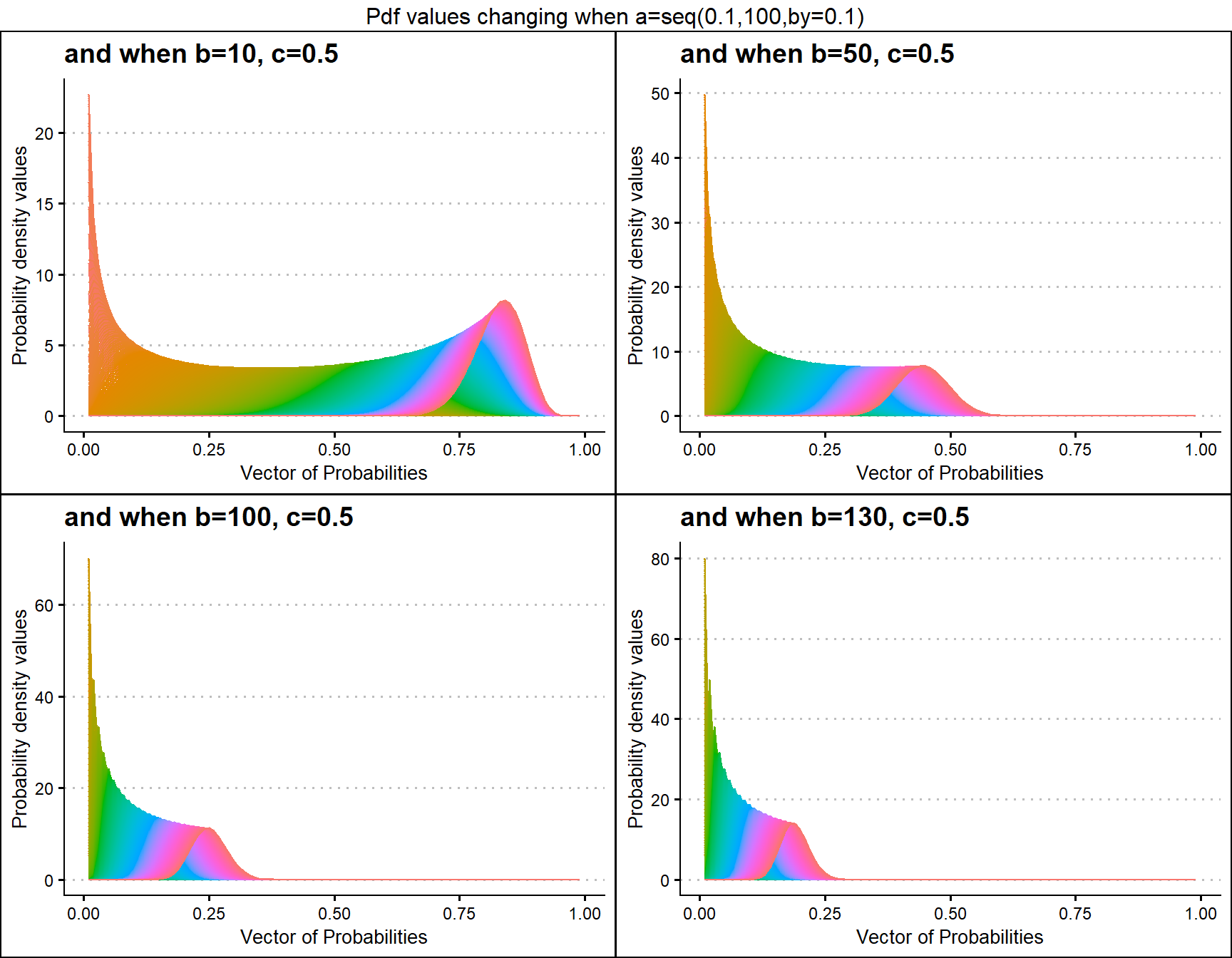
 b10c1 <- dGBeta1plot(a=seq(.1,100,by=.1),b=10,c=1,
                   plot_title="and when b=10, c=1",a_seq=T,b_seq=F)
 b50c1 <- dGBeta1plot(a=seq(.1,100,by=.1),b=50,c=1,
                   plot_title="and when b=50, c=1",a_seq=T,b_seq=F)
b100c1 <- dGBeta1plot(a=seq(.1,100,by=.1),b=100,c=1,
                    plot_title="and when b=100, c=1",a_seq=T,b_seq=F)
b130c1 <- dGBeta1plot(a=seq(.1,100,by=.1),b=130,c=1,
                    plot_title="and when b=130, c=1",a_seq=T,b_seq=F)

grid.arrange(b10c1,b50c1,b100c1,b130c1,nrow=2,
             top="Pdf values changing when a=seq(0.1,100,by=0.1)")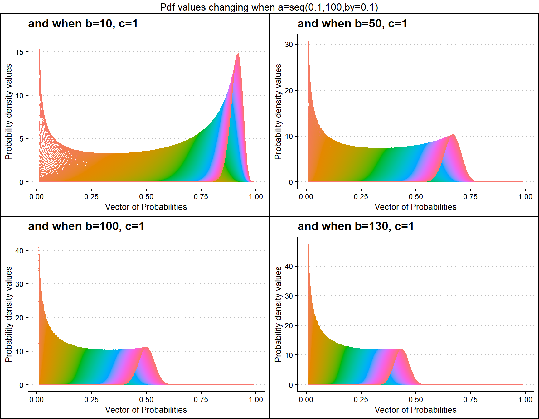
 b10c5 <- dGBeta1plot(a=seq(.1,100,by=.1),b=10,c=5,
                   plot_title="and when b=10, c=5",a_seq=T,b_seq=F)
 b50c5 <- dGBeta1plot(a=seq(.1,100,by=.1),b=50,c=5,
                   plot_title="and when b=50, c=5",a_seq=T,b_seq=F)
b100c5 <- dGBeta1plot(a=seq(.1,100,by=.1),b=100,c=5,
                    plot_title="and when b=100, c=5",a_seq=T,b_seq=F)
b150c5 <- dGBeta1plot(a=seq(.1,100,by=.1),b=150,c=5,
                    plot_title="and when b=150, c=5",a_seq=T,b_seq=F)

grid.arrange(b10c5,b50c5,b100c5,b150c5,nrow=2,
             top="Pdf values changing when a=a=seq(0.1,100,by=0.1)")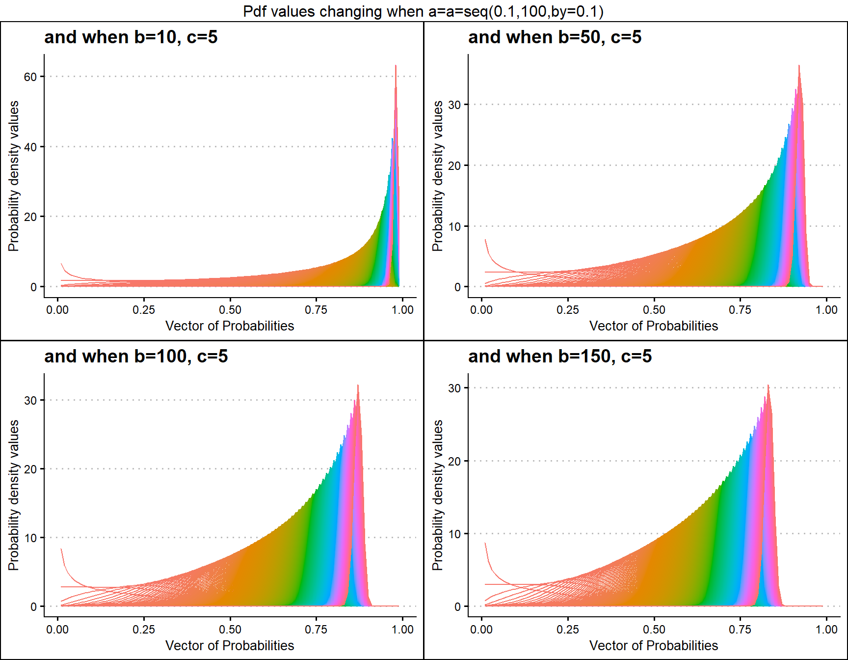
 b10c10 <- dGBeta1plot(a=seq(.1,100,by=.1),b=10,c=10,
                    plot_title="and when b=10, c=10",a_seq=T,b_seq=F)
 b50c10 <- dGBeta1plot(a=seq(.1,100,by=.1),b=50,c=10,
                    plot_title="and when b=50, c=10",a_seq=T,b_seq=F)
b100c10 <- dGBeta1plot(a=seq(.1,100,by=.1),b=100,c=10,
                     plot_title="and when b=100, c=10",a_seq=T,b_seq=F)
b200c10 <- dGBeta1plot(a=seq(.1,100,by=.1),b=200,c=10,
                     plot_title="and when b=200, c=10",a_seq=T,b_seq=F)

grid.arrange(b10c10,b50c10,b100c10,b200c10,nrow=2,
             top="Pdf values changing when a=seq(0.1,100,by=0.1)")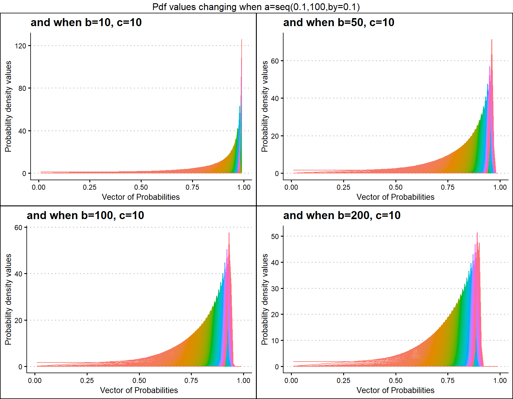
Probability Density values for Gamma Distribution
Gamma distribution has two shape parameters that are a and b. Plots have been generated where with a,b values change and pdf values too.
- a,b are in the domain region of above zero.
b10 <- dGAMMAplot(a=seq(1,100,by=1),b=10,plot_title="and when b=10",a_seq= T)
b50 <- dGAMMAplot(a=seq(1,100,by=1),b=50,plot_title="and when b=50",a_seq= T)
b20 <- dGAMMAplot(a=seq(1,100,by=1),b=20,plot_title="and when b=20",a_seq= T)
b30 <- dGAMMAplot(a=seq(1,100,by=1),b=30,plot_title="and when b=30",a_seq= T)

grid.arrange(b10,b20,b30,b50,nrow=2,top="Pdf values changing when a=seq(1:100,by=1)")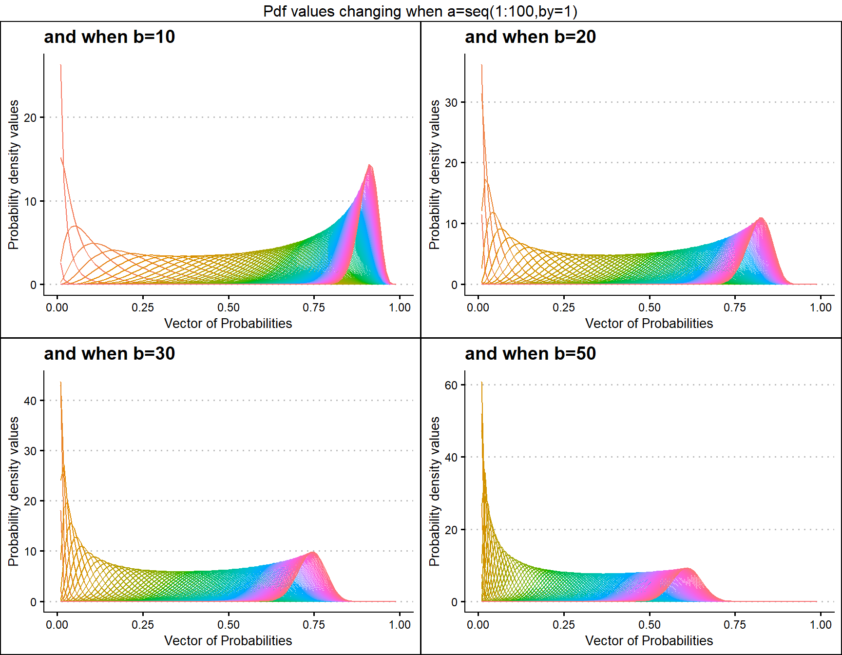
a10 <- dGAMMAplot(b=seq(1,100,by=1),a=10,plot_title="and when a=10",a_seq= F)
a50 <- dGAMMAplot(b=seq(1,100,by=1),a=50,plot_title="and when a=50",a_seq= F)
a20 <- dGAMMAplot(b=seq(1,100,by=1),a=20,plot_title="and when a=20",a_seq= F)
a30 <- dGAMMAplot(b=seq(1,100,by=1),a=30,plot_title="and when a=30",a_seq= F)

grid.arrange(a10,a20,a30,a50,nrow=2,top="Pdf values changing when b=seq(1:100,by=1)")