Triangular Binomial Distribution

These functions provide the ability for generating probability function values and cumulative probability function values for the Triangular Binomial distribution.

dTriBin(x,n,mode)

Arguments

x	vector of binomial random variables.
n	single value for no of binomial trials.
mode	single value for mode.

Value

The output of dTriBin gives a list format consisting

pdf probability function values in vector form.

mean mean of the Triangular Binomial Distribution.

var variance of the Triangular Binomial Distribution.

over.dis.para over dispersion value of the Triangular Binomial Distribution.

Details

Mixing unit bounded Triangular distribution with Binomial distribution will create Triangular Binomial distribution. The probability function and cumulative probability function can be constructed and are denoted below.

The cumulative probability function is the summation of probability function values.

$$P_{TriBin}(x)= 2 {n \choose x}(c^{-1}B_c(x+2,n-x+1)+(1-c)^{-1}B(x+1,n-x+2)-(1-c)^{-1}B_c(x+1,n-x+2))$$ $$0 < mode=c < 1$$ $$x = 0,1,2,...n$$ $$n = 1,2,3...$$

The mean, variance and over dispersion are denoted as $$E_{TriiBin}[x]= \frac{n(1+c)}{3} $$ $$Var_{TriBin}[x]= \frac{n(n+3)}{18}-\frac{n(n-3)c(1-c)}{18} $$ $$over dispersion= \frac{(1-c+c^2)}{2(2+c-c^2)} $$

Defined as \(B_c(a,b)=\int^c_0 t^{a-1} (1-t)^{b-1} \,dt\) is incomplete beta integrals and \(B(a,b)\) is the beta function.

NOTE : If input parameters are not in given domain conditions necessary error messages will be provided to go further.

References

Horsnell, G. (1957). Economic acceptance sampling schemes. Journal of the Royal Statistical Society, Series A, 120:148-191.

Karlis, D. & Xekalaki, E., 2008. The Polygonal Distribution. In Advances in Mathematical and Statistical Modeling. Boston: Birkhuser Boston, pp. 21-33.

Available at: http://dx.doi.org/10.1007/978-0-8176-4626-4_2 .

Okagbue, H. et al., 2014. Using the Average of the Extreme Values of a Triangular Distribution for a Transformation, and Its Approximant via the Continuous Uniform Distribution. British Journal of Mathematics & Computer Science, 4(24), pp.3497-3507.

Available at: http://www.sciencedomain.org/abstract.php?iid=699&id=6&aid=6427.

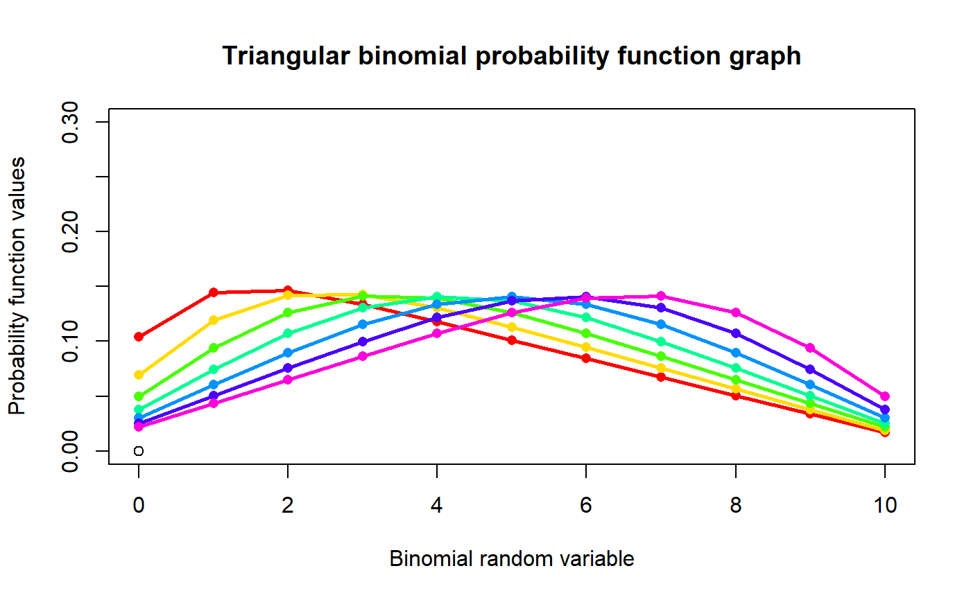
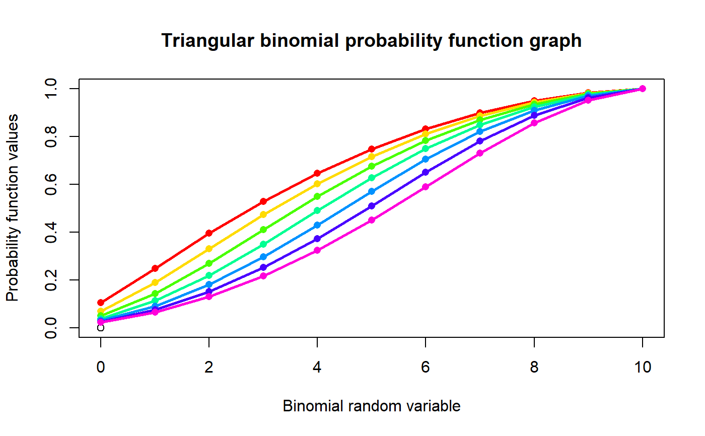
Examples

#plotting the random variables and probability values
col <- rainbow(7)
x <- seq(0.1,0.7,by=0.1)
plot(0,0,main="Triangular binomial probability function graph",xlab="Binomial random variable",
ylab="Probability function values",xlim = c(0,10),ylim = c(0,.3))
for (i in 1:7)
{
lines(0:10,dTriBin(0:10,10,x[i])$pdf,col = col[i],lwd=2.85)
points(0:10,dTriBin(0:10,10,x[i])$pdf,col = col[i],pch=16)
}

dTriBin(0:10,10,.4)$pdf        #extracting the pdf values
#>  [1] 0.03774136 0.07438334 0.10699425 0.13064720 0.14086322 0.13674651
#>  [7] 0.12148214 0.09984766 0.07555898 0.05048387 0.02525147
dTriBin(0:10,10,.4)$mean       #extracting the mean
#> [1] 4.666667
dTriBin(0:10,10,.4)$var        #extracting the variance
#> [1] 6.288889
dTriBin(0:10,10,.4)$over.dis.para  #extracting the over dispersion value
#> [1] 0.1696429

#plotting the random variables and cumulative probability values
col <- rainbow(7)
x <- seq(0.1,0.7,by=0.1)
plot(0,0,main="Triangular binomial probability function graph",xlab="Binomial random variable",
ylab="Probability function values",xlim = c(0,10),ylim = c(0,1))
for (i in 1:7)
{
lines(0:10,pTriBin(0:10,10,x[i]),col = col[i],lwd=2.85)
points(0:10,pTriBin(0:10,10,x[i]),col = col[i],pch=16)
}

pTriBin(0:10,10,.4)    #acquiring the cumulative probability values
#>  [1] 0.03774136 0.11212471 0.21911896 0.34976615 0.49062937 0.62737588
#>  [7] 0.74885802 0.84870568 0.92426467 0.97474853 1.00000000