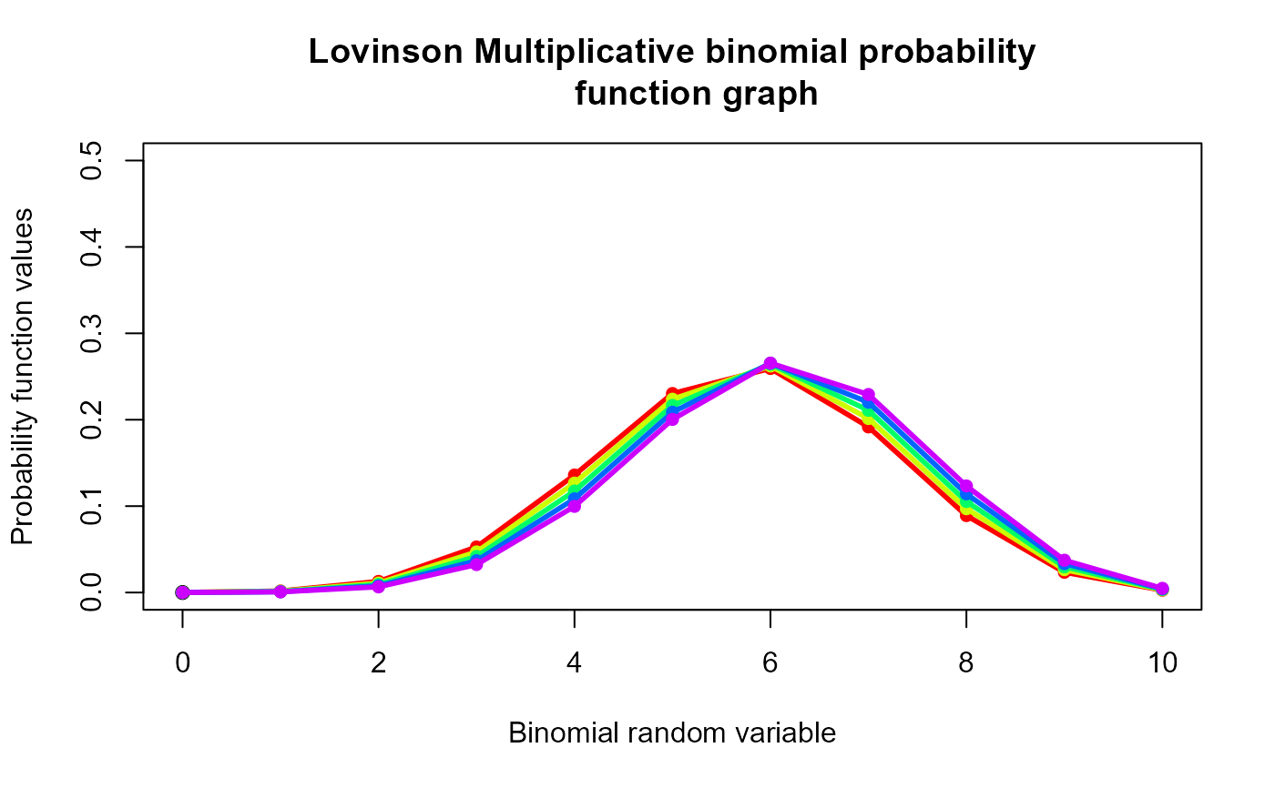
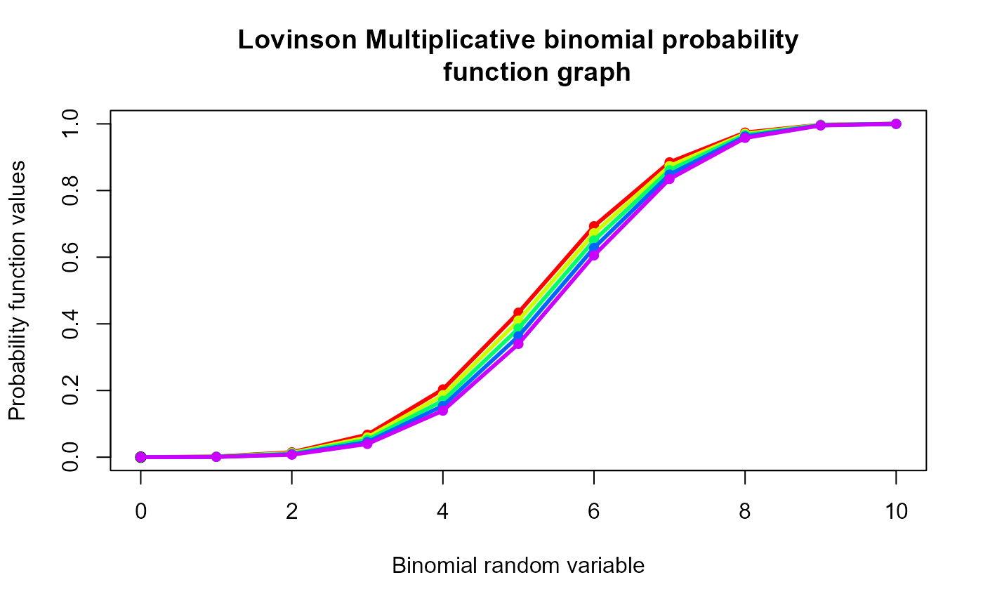
These functions provide the ability for generating probability function values and cumulative probability function values for the Lovinson Multiplicative Binomial Distribution.
Arguments
- x
vector of binomial random variables.
- n
single value for no of binomial trials.
- p
single value for probability of success.
- phi
single value for phi.
Details
The probability function and cumulative function can be constructed and are denoted below
The cumulative probability function is the summation of probability function values.
$$P_{LMBin}(x)= {n \choose x} p^x (1-p)^{n-x} \frac{(phi^{x(n-x)}}{f(p,phi,n)} $$
here \(f(p,phi,n)\) is $$f(p,phi,n)= \sum_{k=0}^{n} {n \choose k} p^k (1-p)^{n-k} (phi^{k(n-k)} )$$
$$x = 0,1,2,3,...n$$ $$n = 1,2,3,...$$ $$k = 0,1,2,...,n$$ $$0 < p < 1$$ $$0 < phi $$
NOTE : If input parameters are not in given domain conditions necessary error messages will be provided to go further.
References
Elamir EA (2013). “Multiplicative-Binomial Distribution: Some Results on Characterization, Inference and Random Data Generation.” Journal of Statistical Theory and Applications, 12(1), 92--105.
Examples
#plotting the random variables and probability values
col <- rainbow(5)
a <- c(0.58,0.59,0.6,0.61,0.62)
b <- c(0.022,0.023,0.024,0.025,0.026)
plot(0,0,main="Lovinson Multiplicative binomial probability
     function graph",xlab="Binomial random variable",
     ylab="Probability function values",xlim = c(0,10),ylim = c(0,0.5))
for (i in 1:5)
{
lines(0:10,dLMBin(0:10,10,a[i],1+b[i])$pdf,col = col[i],lwd=2.85)
points(0:10,dLMBin(0:10,10,a[i],1+b[i])$pdf,col = col[i],pch=16)
}


dLMBin(0:10,10,.58,10.022)$pdf   #extracting the pdf values
#>  [1] 6.364309e-29 8.964365e-19 5.657070e-11 2.106255e-05 5.123785e-02
#>  [6] 8.509524e-01 9.771209e-02 7.659947e-05 3.923411e-10 1.185630e-17
#> [11] 1.605234e-27
dLMBin(0:10,10,.58,10.022)$mean   #extracting the mean
#> [1] 5.046585
dLMBin(0:10,10,.58,10.022)$var   #extracting the variance
#> [1] 0.1471704

#plotting random variables and cumulative probability values
col <- rainbow(5)
a <- c(0.58,0.59,0.6,0.61,0.62)
b <- c(0.022,0.023,0.024,0.025,0.026)
plot(0,0,main="Lovinson Multiplicative binomial probability
     function graph",xlab="Binomial random variable",
     ylab="Probability function values",xlim = c(0,10),ylim = c(0,1))
for (i in 1:5)
{
lines(0:10,pLMBin(0:10,10,a[i],1+b[i]),col = col[i],lwd=2.85)
points(0:10,pLMBin(0:10,10,a[i],1+b[i]),col = col[i],pch=16)
}


pLMBin(0:10,10,.58,10.022)     #acquiring the cumulative probability values
#>  [1] 6.364309e-29 8.964365e-19 5.657070e-11 2.106261e-05 5.125891e-02
#>  [6] 9.022113e-01 9.999234e-01 1.000000e+00 1.000000e+00 1.000000e+00
#> [11] 1.000000e+00
