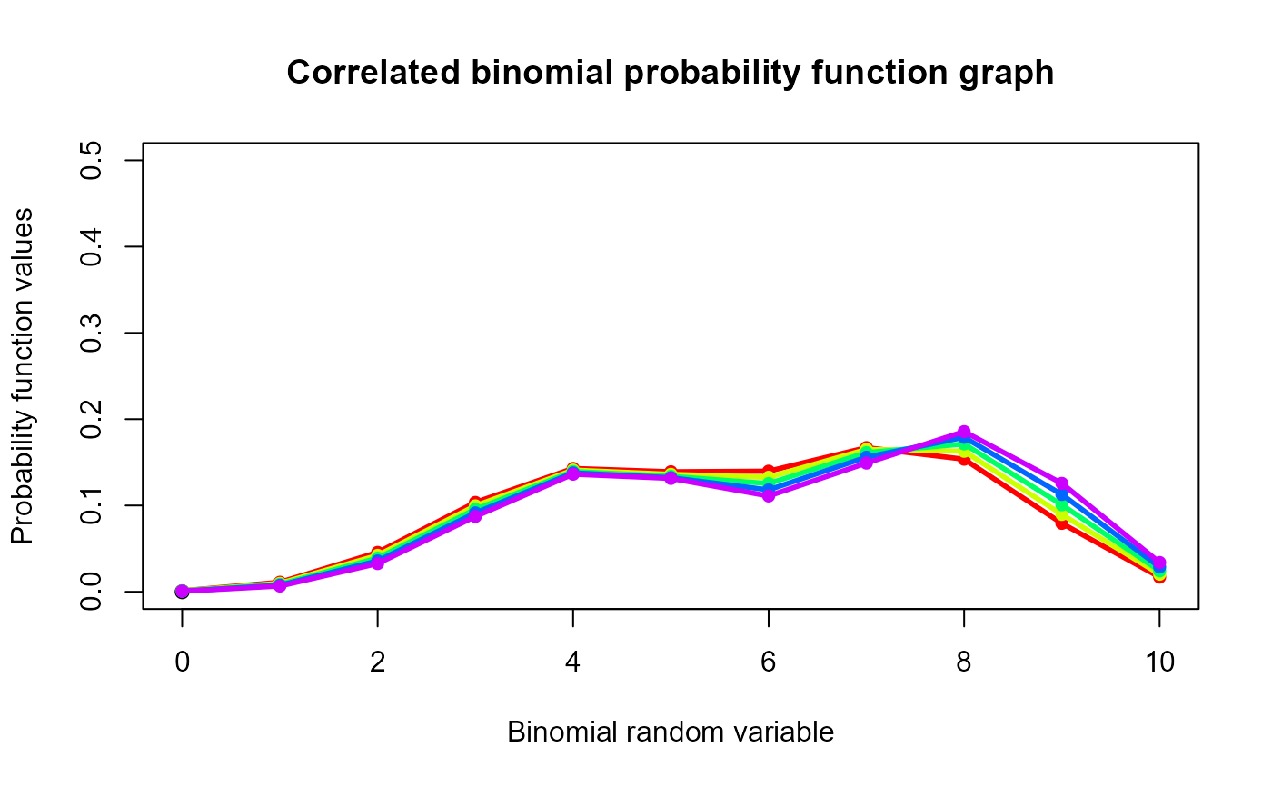
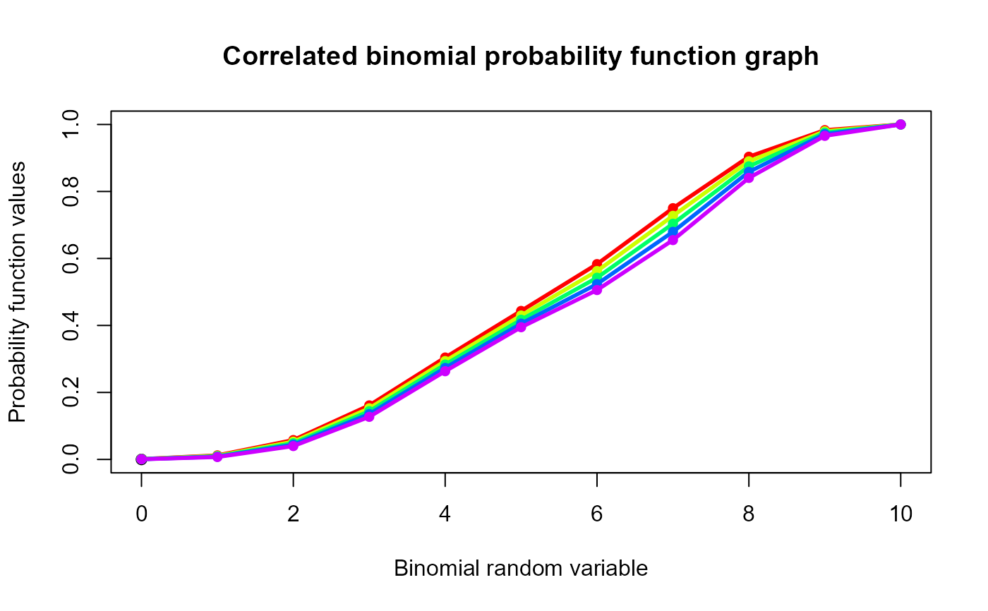
These functions provide the ability for generating probability function values and cumulative probability function values for the Correlated Binomial Distribution.
Arguments
- x
vector of binomial random variables.
- n
single value for no of binomial trials.
- p
single value for probability of success.
- cov
single value for covariance.
Details
The probability function and cumulative function can be constructed and are denoted below
The cumulative probability function is the summation of probability function values.
$$P_{CorrBin}(x) = {n \choose x}(p^x)(1-p)^{n-x}(1+(\frac{cov}{2p^2(1-p)^2})((x-np)^2+x(2p-1)-np^2)) $$ \(x = 0,1,2,3,...n\) \(n = 1,2,3,...\) \(0 < p < 1\) \(-\infty < cov < +\infty \)
The Correlation is in between $$\frac{-2}{n(n-1)} min(\frac{p}{1-p},\frac{1-p}{p}) \le cov \le \frac{2p(1-p)}{(n-1)p(1-p)+0.25-fo} $$ where \(fo=min (x-(n-1)p-0.5)^2 \)
The mean and the variance are denoted as $$E_{CorrBin}[x]= np$$ $$Var_{CorrBin}[x]= n(p(1-p)+(n-1)cov)$$ $$Corr_{CorrBin}[x]=\frac{cov}{p(1-p)}$$
NOTE : If input parameters are not in given domain conditions necessary error messages will be provided to go further.
References
Johnson NL, Kemp AW, Kotz S (2005). Univariate discrete distributions, volume 444. John Wiley and Sons. Kupper LL, Haseman JK (1978). “The use of a correlated binomial model for the analysis of certain toxicological experiments.” Biometrics, 69--76. Paul SR (1985). “A three-parameter generalization of the binomial distribution.” History and Philosophy of Logic, 14(6), 1497--1506. Morel JG, Neerchal NK (2012). Overdispersion models in SAS. SAS Publishing.
Examples
#plotting the random variables and probability values
col <- rainbow(5)
a <- c(0.58,0.59,0.6,0.61,0.62)
b <- c(0.022,0.023,0.024,0.025,0.026)
plot(0,0,main="Correlated binomial probability function graph",xlab="Binomial random variable",
ylab="Probability function values",xlim = c(0,10),ylim = c(0,0.5))
for (i in 1:5)
{
lines(0:10,dCorrBin(0:10,10,a[i],b[i])$pdf,col = col[i],lwd=2.85)
points(0:10,dCorrBin(0:10,10,a[i],b[i])$pdf,col = col[i],pch=16)
}


dCorrBin(0:10,10,0.58,0.022)$pdf      #extracting the pdf values
#>  [1] 0.001129385 0.011031584 0.045621336 0.103565540 0.142922006 0.139070090
#>  [7] 0.139751296 0.167045868 0.153590546 0.079286062 0.016986287
dCorrBin(0:10,10,0.58,0.022)$mean     #extracting the mean
#> [1] 5.8
dCorrBin(0:10,10,0.58,0.022)$var      #extracting the variance
#> [1] 4.416
dCorrBin(0:10,10,0.58,0.022)$corr     #extracting the correlation
#> [1] 0.09031199
dCorrBin(0:10,10,0.58,0.022)$mincorr  #extracting the minimum correlation value
#> [1] -0.01609195
dCorrBin(0:10,10,0.58,0.022)$maxcorr  #extracting the maximum correlation value
#> [1] 0.2060914

#plotting the random variables and cumulative probability values
col <- rainbow(5)
a <- c(0.58,0.59,0.6,0.61,0.62)
b <- c(0.022,0.023,0.024,0.025,0.026)
plot(0,0,main="Correlated binomial probability function graph",xlab="Binomial random variable",
ylab="Probability function values",xlim = c(0,10),ylim = c(0,1))
for (i in 1:5)
{
lines(0:10,pCorrBin(0:10,10,a[i],b[i]),col = col[i],lwd=2.85)
points(0:10,pCorrBin(0:10,10,a[i],b[i]),col = col[i],pch=16)
}


pCorrBin(0:10,10,0.58,0.022)      #acquiring the cumulative probability values
#>  [1] 0.001129385 0.012160968 0.057782305 0.161347845 0.304269851 0.443339941
#>  [7] 0.583091237 0.750137105 0.903727651 0.983013713 1.000000000
