These functions provide the ability for generating probability function values and cumulative probability function values for the Beta-Binomial Distribution.
Arguments
- x
vector of binomial random variables.
- n
single value for no of binomial trials.
- a
single value for shape parameter alpha representing as a.
- b
single value for shape parameter beta representing as b.
Value
The output of dBetaBin gives a list format consisting
pdf probability function values in vector form.
mean mean of the Beta-Binomial Distribution.
var variance of the Beta-Binomial Distribution.
over.dis.para over dispersion value of the Beta-Binomial Distribution.
Details
Mixing Beta distribution with Binomial distribution will create the Beta-Binomial distribution. The probability function and cumulative probability function can be constructed and are denoted below.
The cumulative probability function is the summation of probability function values.
$$P_{BetaBin}(x)= {n \choose x} \frac{B(a+x,n+b-x)}{B(a,b)} $$ $$a,b > 0$$ $$x = 0,1,2,3,...n$$ $$n = 1,2,3,...$$
The mean, variance and over dispersion are denoted as $$E_{BetaBin}[x]= \frac{na}{a+b} $$ $$Var_{BetaBin}[x]= \frac{(nab)}{(a+b)^2} \frac{(a+b+n)}{(a+b+1)} $$ $$over dispersion= \frac{1}{a+b+1} $$
Defined as B(a,b) is the beta function.
References
Young-Xu Y, Chan KA (2008). “Pooling overdispersed binomial data to estimate event rate.” BMC medical research methodology, 8, 1--12. Trenkler G (1996). “Continuous univariate distributions.” Computational Statistics and Data Analysis, 21(1), 119--119. HUGHES G, MADDEN L (1993). “Using the beta-binomial distribution to describe aggegated patterns of disease incidence.” Phytopathology, 83(7), 759--763.
Examples
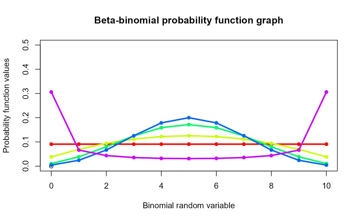
#plotting the random variables and probability values
col <- rainbow(5)
a <- c(1,2,5,10,0.2)
plot(0,0,main="Beta-binomial probability function graph",xlab="Binomial random variable",
ylab="Probability function values",xlim = c(0,10),ylim = c(0,0.5))
for (i in 1:5)
{
lines(0:10,dBetaBin(0:10,10,a[i],a[i])$pdf,col = col[i],lwd=2.85)
points(0:10,dBetaBin(0:10,10,a[i],a[i])$pdf,col = col[i],pch=16)
}
 dBetaBin(0:10,10,4,.2)$pdf #extracting the pdf values
#> [1] 9.184001e-05 3.993044e-04 1.095652e-03 2.434783e-03 4.810660e-03
#> [6] 8.881218e-03 1.585932e-02 2.832021e-02 5.310040e-02 1.180009e-01
#> [11] 7.670057e-01
dBetaBin(0:10,10,4,.2)$mean #extracting the mean
#> [1] 9.52381
dBetaBin(0:10,10,4,.2)$var #extracting the variance
#> [1] 1.238444
dBetaBin(0:10,10,4,.2)$over.dis.para #extracting the over dispersion value
#> [1] 0.1923077
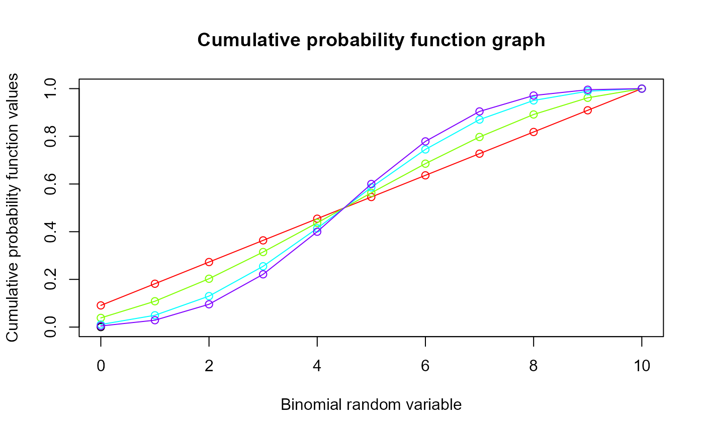
#plotting the random variables and cumulative probability values
col <- rainbow(4)
a <- c(1,2,5,10)
plot(0,0,main="Cumulative probability function graph",xlab="Binomial random variable",
ylab="Cumulative probability function values",xlim = c(0,10),ylim = c(0,1))
for (i in 1:4)
{
lines(0:10,pBetaBin(0:10,10,a[i],a[i]),col = col[i])
points(0:10,pBetaBin(0:10,10,a[i],a[i]),col = col[i])
}
dBetaBin(0:10,10,4,.2)$pdf #extracting the pdf values
#> [1] 9.184001e-05 3.993044e-04 1.095652e-03 2.434783e-03 4.810660e-03
#> [6] 8.881218e-03 1.585932e-02 2.832021e-02 5.310040e-02 1.180009e-01
#> [11] 7.670057e-01
dBetaBin(0:10,10,4,.2)$mean #extracting the mean
#> [1] 9.52381
dBetaBin(0:10,10,4,.2)$var #extracting the variance
#> [1] 1.238444
dBetaBin(0:10,10,4,.2)$over.dis.para #extracting the over dispersion value
#> [1] 0.1923077
#plotting the random variables and cumulative probability values
col <- rainbow(4)
a <- c(1,2,5,10)
plot(0,0,main="Cumulative probability function graph",xlab="Binomial random variable",
ylab="Cumulative probability function values",xlim = c(0,10),ylim = c(0,1))
for (i in 1:4)
{
lines(0:10,pBetaBin(0:10,10,a[i],a[i]),col = col[i])
points(0:10,pBetaBin(0:10,10,a[i],a[i]),col = col[i])
}
 pBetaBin(0:10,10,4,.2) #acquiring the cumulative probability values
#> [1] 9.184001e-05 4.911444e-04 1.586797e-03 4.021580e-03 8.832240e-03
#> [6] 1.771346e-02 3.357278e-02 6.189299e-02 1.149934e-01 2.329943e-01
#> [11] 1.000000e+00
pBetaBin(0:10,10,4,.2) #acquiring the cumulative probability values
#> [1] 9.184001e-05 4.911444e-04 1.586797e-03 4.021580e-03 8.832240e-03
#> [6] 1.771346e-02 3.357278e-02 6.189299e-02 1.149934e-01 2.329943e-01
#> [11] 1.000000e+00