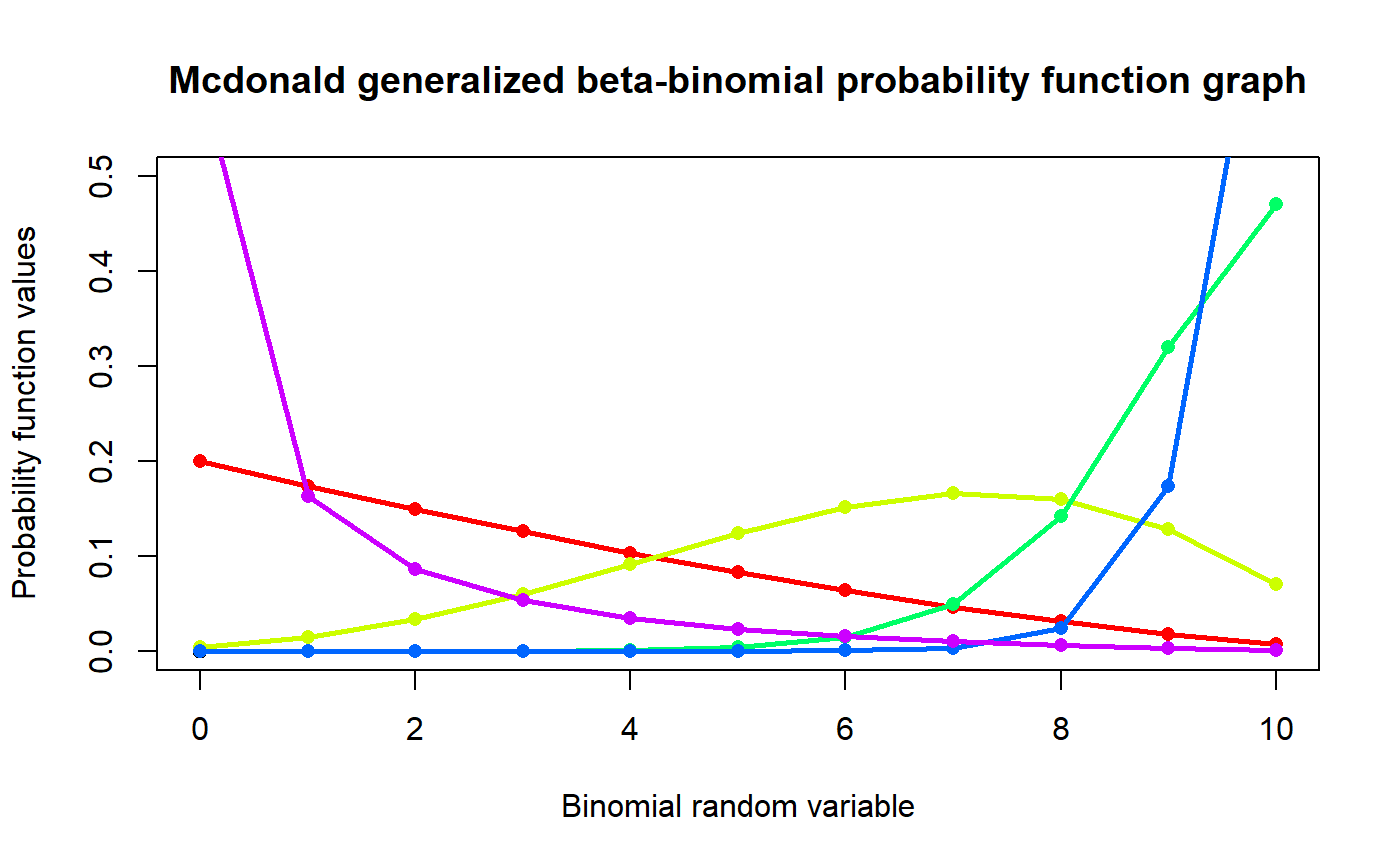
These functions provide the ability for generating probability function values and cumulative probability function values for the McDonald Generalized Beta Binomial Distribution.
pMcGBB(x,n,a,b,c)
Arguments
| x | vector of binomial random variables. |
|---|---|
| n | single value for no of binomial trials. |
| a | single value for shape parameter alpha representing as a. |
| b | single value for shape parameter beta representing as b. |
| c | single value for shape parameter gamma representing as c. |
Value
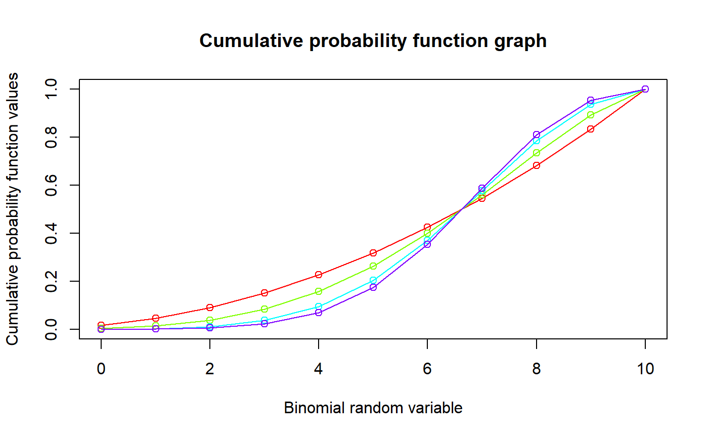
The output of pMcGBB gives cumulative probability function values in vector form.
Details
Mixing Generalized Beta Type-1 Distribution with Binomial distribution the probability function value and cumulative probability function can be constructed and are denoted below.
The cumulative probability function is the summation of probability function values.
$$P_{McGBB}(x)= {n \choose x} \frac{1}{B(a,b)} (\sum_{j=0}^{n-x} (-1)^j {n-x \choose j} B(\frac{x}{c}+a+\frac{j}{c},b) ) $$ $$a,b,c > 0$$
The mean, variance and over dispersion are denoted as $$E_{McGBB}[x]= n\frac{B(a+b,\frac{1}{c})}{B(a,\frac{1}{c})} $$ $$Var_{McGBB}[x]= n^2(\frac{B(a+b,\frac{2}{c})}{B(a,\frac{2}{c})}-(\frac{B(a+b,\frac{1}{c})}{B(a,\frac{1}{c})})^2) +n(\frac{B(a+b,\frac{1}{c})}{B(a,\frac{1}{c})}-\frac{B(a+b,\frac{2}{c})}{B(a,\frac{2}{c})}) $$ $$over dispersion= \frac{\frac{B(a+b,\frac{2}{c})}{B(a,\frac{2}{c})}-(\frac{B(a+b,\frac{1}{c})}{B(a,\frac{1}{c})})^2}{\frac{B(a+b,\frac{1}{c})}{B(a,\frac{1}{c})}-(\frac{B(a+b,\frac{1}{c})}{B(a,\frac{1}{c})})^2}$$ $$x = 0,1,2,...n$$ $$n = 1,2,3,...$$
References
Manoj, C., Wijekoon, P. & Yapa, R.D., 2013. The McDonald Generalized Beta-Binomial Distribution: A New Binomial Mixture Distribution and Simulation Based Comparison with Its Nested Distributions in Handling Overdispersion. International Journal of Statistics and Probability, 2(2), pp.24-41.
Available at: http://www.ccsenet.org/journal/index.php/ijsp/article/view/23491.
Janiffer, N.M., Islam, A. & Luke, O., 2014. Estimating Equations for Estimation of Mcdonald Generalized Beta - Binomial Parameters. , (October), pp.702-709.
Roozegar, R., Tahmasebi, S. & Jafari, A.A., 2015. The McDonald Gompertz Distribution: Properties and Applications. Communications in Statistics - Simulation and Computation, (May), pp.0-0.
Available at: http://www.tandfonline.com/doi/full/10.1080/03610918.2015.1088024.
Examples
#plotting the random variables and probability values col <- rainbow(5) a <- c(1,2,5,10,0.6) plot(0,0,main="Mcdonald generalized beta-binomial probability function graph", xlab="Binomial random variable",ylab="Probability function values",xlim = c(0,10),ylim = c(0,0.5))for (i in 1:5) { lines(0:10,dMcGBB(0:10,10,a[i],2.5,a[i])$pdf,col = col[i],lwd=2.85) points(0:10,dMcGBB(0:10,10,a[i],2.5,a[i])$pdf,col = col[i],pch=16) }#> [1] 0.003663004 0.013320013 0.029970030 0.053280053 0.081585082 0.111888112 #> [7] 0.139860140 0.159840160 0.164835165 0.146520147 0.095238095#> [1] 6.666667#> [1] 3.174603#> [1] 0.1428571#plotting the random variables and cumulative probability values col <- rainbow(4) a <- c(1,2,5,10) plot(0,0,main="Cumulative probability function graph",xlab="Binomial random variable", ylab="Cumulative probability function values",xlim = c(0,10),ylim = c(0,1))for (i in 1:4) { lines(0:10,pMcGBB(0:10,10,a[i],a[i],2),col = col[i]) points(0:10,pMcGBB(0:10,10,a[i],a[i],2),col = col[i]) }pMcGBB(0:10,10,4,2,1) #acquiring the cumulative probability values#> [1] 0.003663004 0.016983017 0.046953047 0.100233100 0.181818182 0.293706294 #> [7] 0.433566434 0.593406593 0.758241758 0.904761905 1.000000000