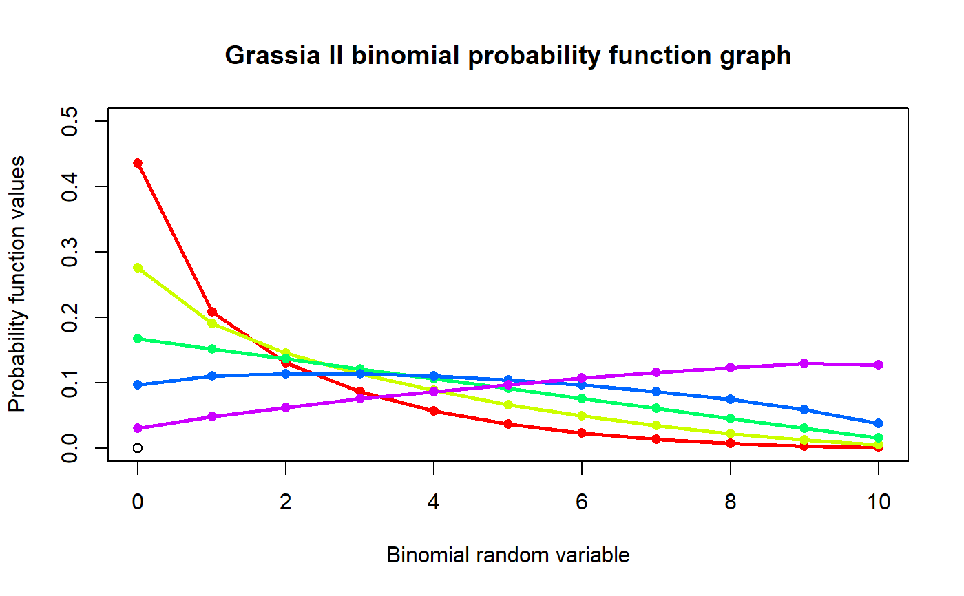
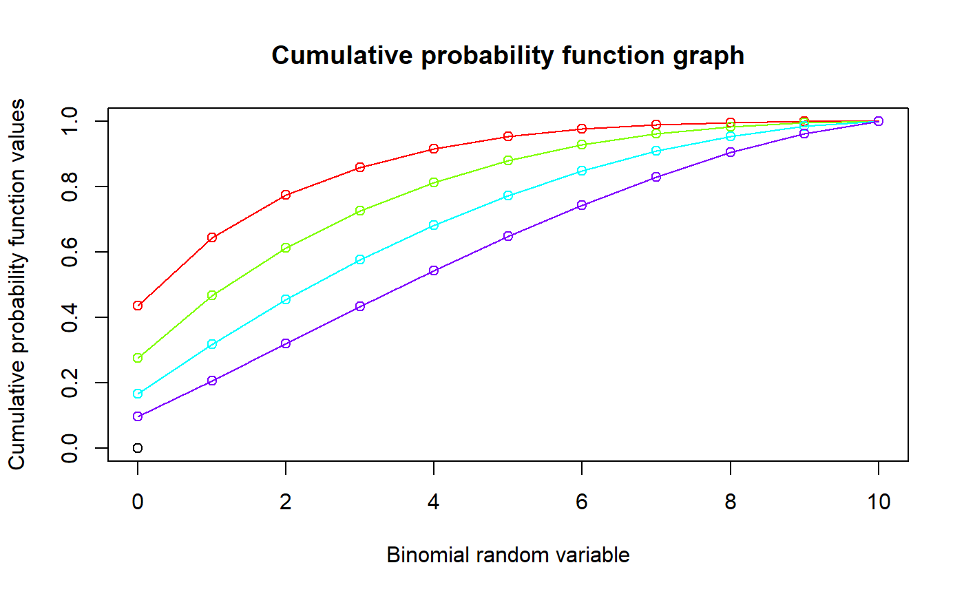
These functions provide the ability for generating probability function values and cumulative probability function values for the Grassia-II-Binomial Distribution.
pGrassiaIIBin(x,n,a,b)
Arguments
| x | vector of binomial random variables. |
|---|---|
| n | single value for no of binomial trials. |
| a | single value for shape parameter a. |
| b | single value for shape parameter b. |
Value
The output of pGrassiaIIBin gives cumulative probability values in vector form.
Details
Mixing Gamma distribution with Binomial distribution will create the the Grassia-II-Binomial distribution, only when (1-p)=e^(-lambda) of the Binomial distribution. The probability function and cumulative probability function can be constructed and are denoted below.
The cumulative probability function is the summation of probability function values.
$$P_{GrassiaIIBin}[x]= {n \choose x} \sum_{j=0}^{x} {x \choose j} (-1)^{x-j} (1+b(n-j))^{-a} $$ $$a,b > 0$$ $$x = 0,1,2,...,n$$ $$n = 1,2,3,...$$
The mean, variance and over dispersion are denoted as $$E_{GrassiaIIBin}[x] = (\frac{b}{b+1})^a$$ $$Var_{GrassiaIIBin}[x] = n^2[(\frac{b}{b+2})^a - (\frac{b}{b+1})^{2a}] + n(\frac{b}{b+1})^a{1-(\frac{b+1}{b+2})^a}$$ $$over dispersion= \frac{(\frac{b}{b+2})^a - (\frac{b}{b+1})^{2a}}{(\frac{b}{b+1})^a[1-(\frac{b}{b+1})^a]}$$
References
Grassia, A., 1977. On a family of distributions with argument between 0 and 1 obtained by transformation of the gamma and derived compound distributions. Australian Journal of Statistics, 19(2), pp.108-114.
Examples
#plotting the random variables and probability values col <- rainbow(5) a <- c(0.3,0.4,0.5,0.6,0.8) plot(0,0,main="Grassia II binomial probability function graph",xlab="Binomial random variable", ylab="Probability function values",xlim = c(0,10),ylim = c(0,0.5))for (i in 1:5) { lines(0:10,dGrassiaIIBin(0:10,10,2*a[i],a[i])$pdf,col = col[i],lwd=2.85) points(0:10,dGrassiaIIBin(0:10,10,2*a[i],a[i])$pdf,col = col[i],pch=16) }#> [1] 0.01234568 0.03923584 0.07605633 0.11447585 0.14524039 0.16058356 #> [7] 0.15614273 0.13223144 0.09426128 0.05202202 0.01740489#> [1] 0.007716049#> [1] 0.01380363#> [1] 0.0878147#plotting the random variables and cumulative probability values col <- rainbow(4) a <- c(0.3,0.4,0.5,0.6) plot(0,0,main="Cumulative probability function graph",xlab="Binomial random variable", ylab="Cumulative probability function values",xlim = c(0,10),ylim = c(0,1))for (i in 1:4) { lines(0:10,pGrassiaIIBin(0:10,10,2*a[i],a[i]),col = col[i]) points(0:10,pGrassiaIIBin(0:10,10,2*a[i],a[i]),col = col[i]) }pGrassiaIIBin(0:10,10,4,.2) #acquiring the cumulative probability values#> [1] 0.01234568 0.05158152 0.12763785 0.24211370 0.38735409 0.54793764 #> [7] 0.70408037 0.83631181 0.93057309 0.98259511 1.00000000