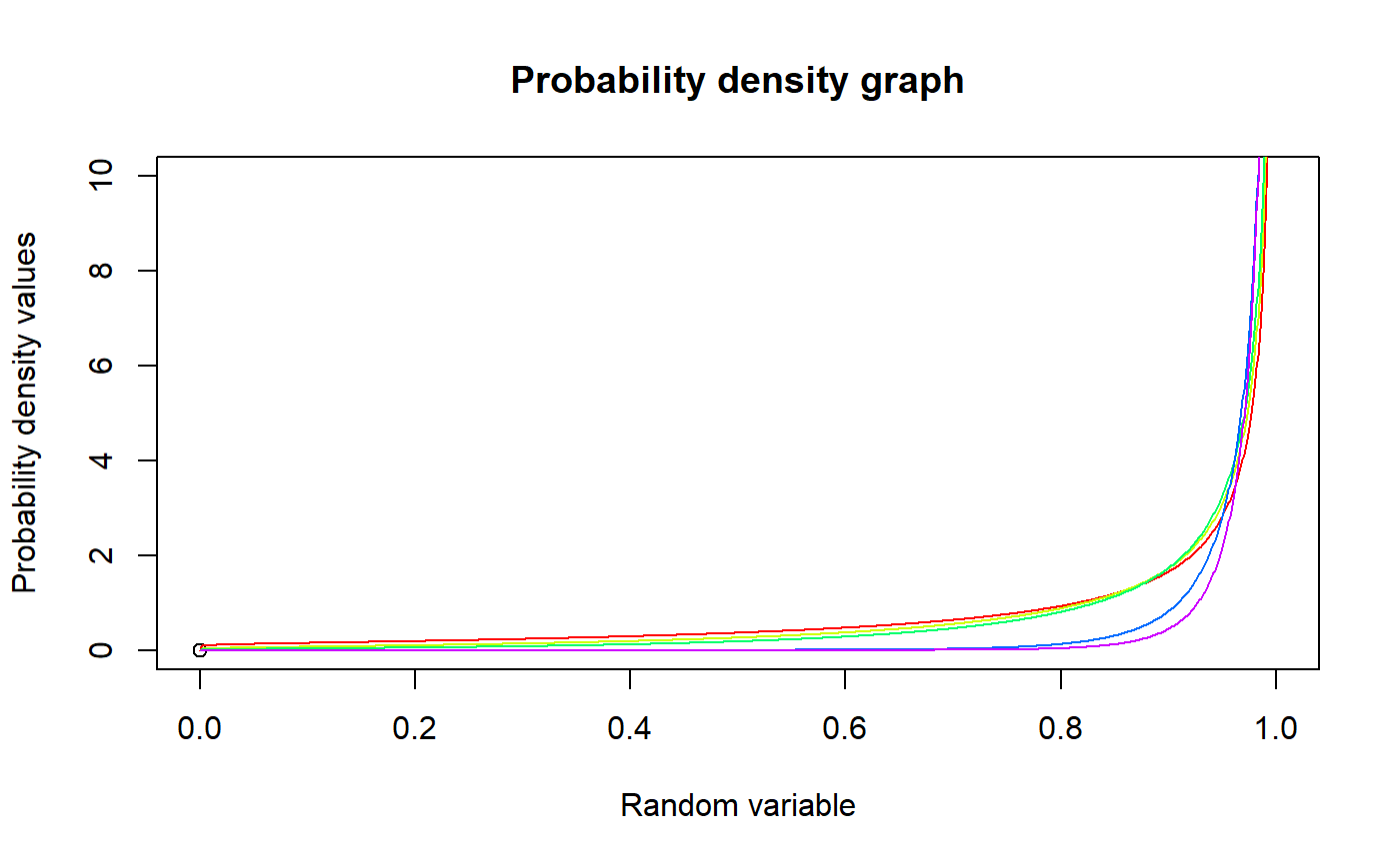
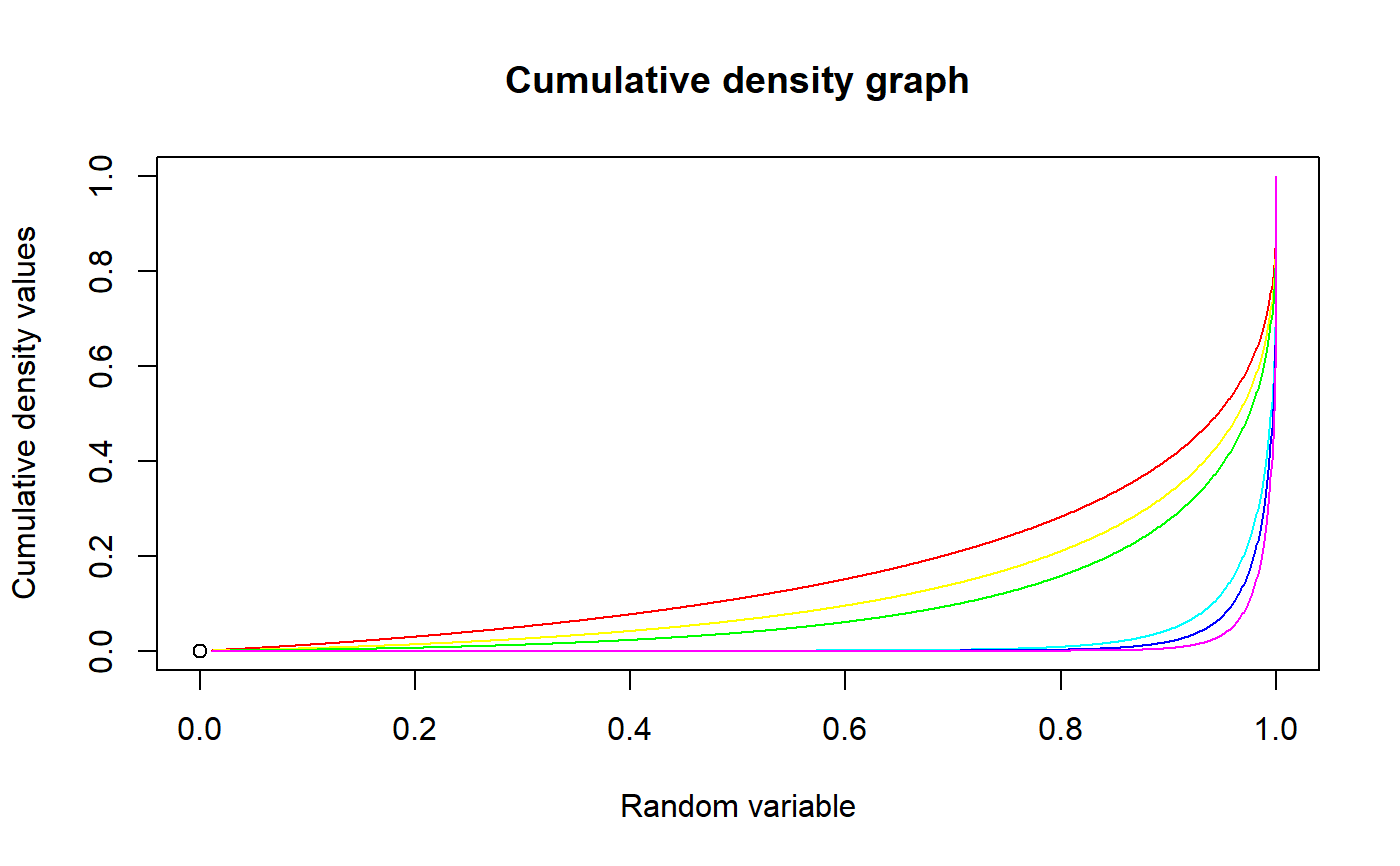
These functions provide the ability for generating probability density values, cumulative probability density values and moment about zero values for the Gaussian Hypergeometric Generalized Beta distribution bounded between [0,1].
pGHGBeta(p,n,a,b,c)
Arguments
| p | vector of probabilities. |
|---|---|
| n | single value for no of binomial trials. |
| a | single value for shape parameter alpha representing as a. |
| b | single value for shape parameter beta representing as b. |
| c | single value for shape parameter lambda representing as c. |
Value
The output of pGHGBeta gives the cumulative density values in vector form.
Details
The probability density function and cumulative density function of a unit bounded Gaussian Hypergeometric Generalized Beta Distribution with random variable P are given by
$$g_{P}(p)= \frac{1}{B(a,b)}\frac{2F1(-n,a;-b-n+1;1)}{2F1(-n,a;-b-n+1;c)} p^{a-1}(1-p)^{b-1} \frac{c^{b+n}}{(c+(1-c)p)^{a+b+n}} $$; \(0 \le p \le 1\) $$G_{P}(p)= \int^p_0 \frac{1}{B(a,b)}\frac{2F1(-n,a;-b-n+1;1)}{2F1(-n,a;-b-n+1;c)} t^{a-1}(1-t)^{b-1}\frac{c^{b+n}}{(c+(1-c)t)^{a+b+n}} \,dt $$ ; \(0 \le p \le 1\) $$a,b,c > 0$$ $$n = 1,2,3,...$$
The mean and the variance are denoted by $$E[P]= \int^1_0 \frac{p}{B(a,b)}\frac{2F1(-n,a;-b-n+1;1)}{2F1(-n,a;-b-n+1;c)} p^{a-1}(1-p)^{b-1}\frac{c^{b+n}}{(c+(1-c)p)^{a+b+n}} \,dp $$ $$var[P]= \int^1_0 \frac{p^2}{B(a,b)}\frac{2F1(-n,a;-b-n+1;1)}{2F1(-n,a;-b-n+1;c)} p^{a-1}(1-p)^{b-1}\frac{c^{b+n}}{(c+(1-c)p)^{a+b+n}} \,dp - (E[p])^2$$
The moments about zero is denoted as $$E[P^r]= \int^1_0 \frac{p^r}{B(a,b)}\frac{2F1(-n,a;-b-n+1;1)}{2F1(-n,a;-b-n+1;c)} p^{a-1}(1-p)^{b-1}\frac{c^{b+n}}{(c+(1-c)p)^{a+b+n}} \,dp$$ \(r = 1,2,3,...\)
Defined as \(B(a,b)\) as the beta function. Defined as \(2F1(a,b;c;d)\) as the Gaussian Hypergeometric function.
NOTE : If input parameters are not in given domain conditions necessary error messages will be provided to go further.
References
Rodriguez-Avi, J., Conde-Sanchez, A., Saez-Castillo, A. J., & Olmo-Jimenez, M. J. (2007). A generalization of the beta-binomial distribution. Journal of the Royal Statistical Society. Series C (Applied Statistics), 56(1), 51-61.
Available at : http://dx.doi.org/10.1111/j.1467-9876.2007.00564.x
Pearson, J., 2009. Computation of Hypergeometric Functions. Transformation, (September), p.1--123.
See also
Examples
#plotting the random variables and probability values col <- rainbow(5) a <- c(.1,.2,.3,1.5,2.15) plot(0,0,main="Probability density graph",xlab="Random variable",ylab="Probability density values", xlim = c(0,1),ylim = c(0,10))for (i in 1:5) { lines(seq(0,1,by=0.001),dGHGBeta(seq(0,1,by=0.001),7,1+a[i],0.3,1+a[i])$pdf,col = col[i]) }#> [1] 0.0000000 0.3509262 0.5228737 0.6498913 0.7501031 0.8314439 0.8984165 #> [8] 0.9539442 1.0000887 1.0383876 1.0700333 1.0959788 1.1170022 1.1337505 #> [15] 1.1467690 1.1565225 1.1634108 1.1677804 1.1699335 1.1701354 1.1686196 #> [22] 1.1655927 1.1612380 1.1557188 1.1491806 1.1417536 1.1335546 1.1246883 #> [29] 1.1152486 1.1053204 1.0949799 1.0842960 1.0733307 1.0621401 1.0507751 #> [36] 1.0392813 1.0277005 1.0160703 1.0044248 0.9927948 0.9812086 0.9696918 #> [43] 0.9582674 0.9469569 0.9357794 0.9247528 0.9138932 0.9032156 0.8927339 #> [50] 0.8824609 0.8724086 0.8625882 0.8530105 0.8436855 0.8346233 0.8258333 #> [57] 0.8173251 0.8091080 0.8011917 0.7935860 0.7863010 0.7793473 0.7727362 #> [64] 0.7664797 0.7605909 0.7550840 0.7499744 0.7452794 0.7410182 0.7372121 #> [71] 0.7338851 0.7310645 0.7287810 0.7270699 0.7259715 0.7255322 0.7258059 #> [78] 0.7268551 0.7287532 0.7315867 0.7354580 0.7404897 0.7468297 0.7546578 #> [85] 0.7641951 0.7757165 0.7895686 0.8061949 0.8261722 0.8502673 0.8795219 #> [92] 0.9153933 0.9599887 1.0164861 1.0899378 1.1889502 1.3296336 1.5465948 #> [99] 1.9327387 2.8776352 Inf#> [1] 0.5279419#> [1] 0.09648382#plotting the random variables and cumulative probability values col <- rainbow(6) a <- c(.1,.2,.3,1.5,2.1,3) plot(0,0,main="Cumulative density graph",xlab="Random variable",ylab="Cumulative density values", xlim = c(0,1),ylim = c(0,1))for (i in 1:6) { lines(seq(0.01,1,by=0.001),pGHGBeta(seq(0.01,1,by=0.001),7,1+a[i],0.3,1+a[i]),col=col[i]) }#> [1] 0.000000000 0.002183554 0.006603937 0.012495083 0.019513343 0.027434627 #> [7] 0.036094544 0.045364862 0.055142153 0.065340545 0.075887778 0.086722256 #> [13] 0.097790990 0.109048005 0.120453512 0.131972520 0.143574429 0.155232357 #> [19] 0.166922664 0.178624540 0.190319663 0.201991911 0.213627107 0.225212805 #> [25] 0.236738102 0.248193470 0.259570533 0.270862265 0.282062393 0.293165615 #> [31] 0.304167434 0.315064076 0.325852422 0.336529945 0.347094650 0.357545024 #> [37] 0.367879993 0.378098877 0.388201355 0.398187430 0.408057404 0.417811841 #> [43] 0.427451554 0.436977576 0.446391143 0.455693674 0.464886762 0.473972152 #> [49] 0.482951735 0.491827534 0.500601696 0.509276404 0.517854193 0.526337459 #> [55] 0.534728782 0.543030835 0.551246389 0.559378309 0.567429555 0.575403182 #> [61] 0.583302347 0.591130309 0.598890438 0.606586219 0.614221261 0.621799313 #> [67] 0.629324268 0.636800185 0.644231304 0.651622068 0.658977145 0.666301461 #> [73] 0.673600228 0.680878991 0.688143671 0.695400620 0.702656694 0.709919325 #> [79] 0.717196627 0.724497509 0.731831821 0.739210537 0.746645976 0.754152090 #> [85] 0.761744827 0.769442602 0.777266920 0.785243211 0.793401970 0.801780355 #> [91] 0.810424473 0.819392782 0.828761308 0.838632034 0.849147177 0.860515236 #> [97] 0.873063293 0.887356913 0.904538189 0.927708021 1.000002698#> [1] 0.5279419#acquiring the variance for a=1.6312,b=0.3913,c=0.6659 mazGHGBeta(2,7,1.6312,0.3913,0.6659)-mazGHGBeta(1,7,1.6312,0.3913,0.6659)^2#> [1] 0.09648382#only the integer value of moments is taken here because moments cannot be decimal mazGHGBeta(1.9,15,5,6,1)#> [1] 0.4545455