These functions provide the ability for generating probability function values and cumulative probability function values for the Gaussian Hypergeometric Generalized Beta Binomial distribution.
pGHGBB(x,n,a,b,c)
Arguments
| x | vector of binomial random variables. |
|---|---|
| n | single value for no of binomial trials. |
| a | single value for shape parameter alpha value representing a. |
| b | single value for shape parameter beta value representing b. |
| c | single value for shape parameter lambda value representing c. |
Value
The output of pGHGBB gives cumulative probability function values in vector form.
Details
Mixing Gaussian Hypergeometric Generalized Beta distribution with Binomial distribution will create the Gaussian Hypergeometric Generalized Beta Binomial distribution. The probability function and cumulative probability function can be constructed and are denoted below.
The cumulative probability function is the summation of probability function values.
$$P_{GHGBB}(x)=\frac{1}{2F1(-n,a;-b-n+1;c)}{n \choose x} \frac{B(x+a,n-x+b)}{B(a,b+n)}(c^x) $$ $$a,b,c > 0$$ $$x = 0,1,2,...n$$ $$n = 1,2,3,...$$
The mean, variance and over dispersion are denoted as $$E_{GHGBB}[x]= nE_{GHGBeta} $$ $$Var_{GHGBB}[x]= nE_{GHGBeta}(1-E_{GHGBeta})+ n(n-1)Var_{GHGBeta} $$ $$over dispersion= \frac{var_{GHGBeta}}{E_{GHGBeta}(1-E_{GHGBeta})} $$
Defined as \(B(a,b)\) is the beta function. Defined as \(2F1(a,b;c;d)\) is the Gaussian Hypergeometric function.
NOTE : If input parameters are not in given domain conditions necessary error messages will be provided to go further.
References
Rodriguez-Avi, J., Conde-Sanchez, A., Saez-Castillo, A. J., & Olmo-Jimenez, M. J. (2007). A generalization of the beta-binomial distribution. Journal of the Royal Statistical Society. Series C (Applied Statistics), 56(1), 51-61.
Available at : http://dx.doi.org/10.1111/j.1467-9876.2007.00564.x
Pearson, J., 2009. Computation of Hypergeometric Functions. Transformation, (September), p.1--123.
See also
Examples
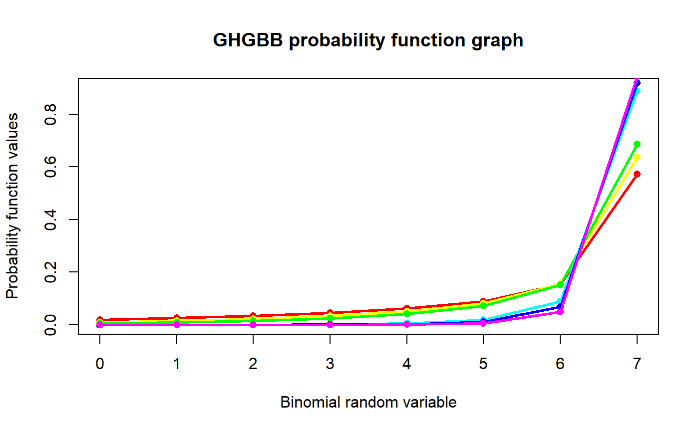
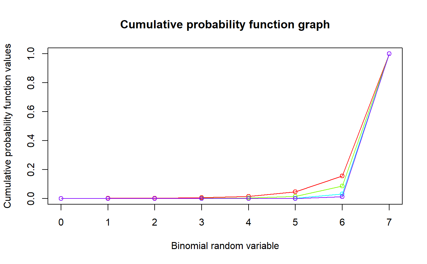
#plotting the random variables and probability values col <- rainbow(6) a <- c(.1,.2,.3,1.5,2.1,3) plot(0,0,main="GHGBB probability function graph",xlab="Binomial random variable", ylab="Probability function values",xlim = c(0,7),ylim = c(0,0.9))for (i in 1:6) { lines(0:7,dGHGBB(0:7,7,1+a[i],0.3,1+a[i])$pdf,col = col[i],lwd=2.85) points(0:7,dGHGBB(0:7,7,1+a[i],0.3,1+a[i])$pdf,col = col[i],pch=16) }#> [1] 0.004487185 0.008425937 0.014260501 0.023712228 0.040167077 0.072195955 #> [7] 0.151611505 0.685139612#> [1] 6.335378#> [1] 1.619291#> [1] 0.2820006#plotting the random variables and cumulative probability values col <- rainbow(4) a <- c(1,2,5,10) plot(0,0,main="Cumulative probability function graph",xlab="Binomial random variable", ylab="Cumulative probability function values",xlim = c(0,7),ylim = c(0,1))for (i in 1:4) { lines(0:7,pGHGBB(0:7,7,1+a[i],0.3,1+a[i]),col = col[i]) points(0:7,pGHGBB(0:7,7,1+a[i],0.3,1+a[i]),col = col[i]) }pGHGBB(0:7,7,1.3,0.3,1.3) #acquiring the cumulative probability values#> [1] 0.004487185 0.012913122 0.027173623 0.050885851 0.091052928 0.163248883 #> [7] 0.314860388 1.000000000